Deep Reinforcement Learning

Multi-armed bandits

Prof. Dr. Sebastian Peitz

Chair of Safe Autonomous Systems, TU Dortmund

Summer term 2026

🚀 by Decker

Content

Multi-armed bandits
Action-value methods
A simple bandit algorithm
What we have not discussed
Some next steps

Example: Route planning (OH16 to Hansaplatz by car)

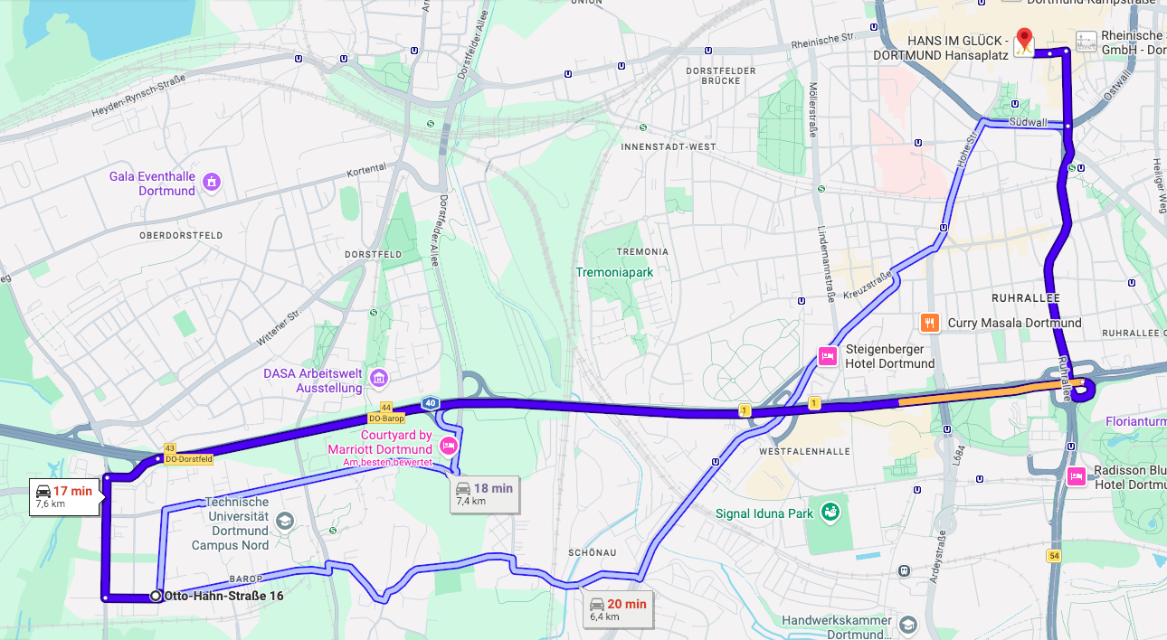
Let’s assume we do not have access to travel time estimates
Which route should I take to minimize my travel time?
Let’s say we can guess the time of one route fairly well
- should we always take this one?
- or try something else and see if we can get better?
This is known as the exploration-exploitation dilemma
The route pickig problem is one example of a multi-armed bandit

Multi-armed bandits

Let us assume that we have a slot machine and we repeatedly can choose between \(k\) different actions
After each choice \(a_t\) you receive a numerical reward \(r_t\) chosen from a stationary probability distribution\(^*\)
Objective: maximize the expected total reward over some time period (e.g., over 1000 action selections, or time steps)
We refer to this as the value: \[ q(a) = \ExpC{r_t}{a_t=a} \]
If we knew \(q(a)\), then it would be easy to choose!
Instead, we have to rely on estimates \(Q_t(a)\) which we can iteratively update based on past experience

Action-value methods

action-value methods: estimate the values of actions and then use these estimates to make action selection decisions
What was the true value again? \(\rightarrow\) the expected reward
What does that mean for a finite number of samples? \(\rightarrow\) we take the mean \[ Q_t(a) = \frac{\sum_{i=1}^{t-1} r_i \cdot \mathbb{1}_{a_i=a}}{\sum_{i=1}^{t-1} \mathbb{1}_{a_i=a}} \] Here, \(\mathbb{1}_{x}\) denotes the random variable that is \(1\) if the predicate \(x\) is true and \(0\) if \(x\) is false. (In other words, we’re counting how often the action \(a\) was taken)
For \(\sum_{i=1}^{t-1} \mathbb{1}_{a_i=a}\) (we have never used the action \(a\)), we can choose a default value such as \(Q_t(a) = 0\)
We call this the sample-average method (Sutton and Barto 1998)

Question: How do we pick the action \(a_t\)? \(\Rightarrow\) just take the max!

\[a_t=\arg\max_a Q_t(a)\]

(with ties broken arbitrarily)

A simple bandit algorithm

The \(k\)-armed testbed

Let’s study a large number of randomly generated \(k\)-armed bandit problems (here: \(k = 10\))
For each bandit problem the action values \(q(a)\), \(a = 1, \ldots, 10\), are selected to a normal distribution: \[ q(a) \sim \Normal{0}{1} \]
The corresponding reward is a random variable as well: \[ r_t \sim \Normal{q(a_t)}{1} \]
One run: perform \(T=1000\) steps. For each time step, report the average reward received until then.
Statistics: repeat the above experiment \(2000\) times

The \(k\)-armed testbed: rewards

First, we are going to follow a greedy strategy: pick the maximizing action always
Then, we will compare against \(\epsilon\) greedy:
- pick the maximizing action \(1-\epsilon\) of the time
- pick a random action \(\epsilon\) of the time

What is \(\epsilon\)’s job? \(\Rightarrow\) the exploration

The \(k\)-armed testbed: optimal actions

Too little (or no) exploration is harmful
Too much exploration is also harmful
Should we think about a schedule in terms of the exploration?

A simple bandit algorithm

# Initialization
for i in range(k):
  Q(a) = 0
  N(a) = 0

# Run forever
while(True):

  # exploration versus exploitation
  if rand() > epsilon:
    a = argmax(Q)        # exploitation
  else:
    a = randint(k)       # exploration

  r = bandit(a)

  # Error correction towards target r 
  N(a) = N(a) + 1
  Q(a) = Q(a) + (1/N(a)) * (r - Q(a))

A simple version of the \(\epsilon\) greedy bandit

Some next steps

Computing \(Q(a)\) on the fly

Calculating \(Q(a)\) anew every time appears to be expensive. For a single action, consider that we have received a sequence of rewards \(r_1,\ldots,r_{t-1}\) so far: \[ Q_t = \frac{r_1 + r_2 + \ldots + r_{t-1}}{t-1}\] Wouldn’t it be easier if we could just updated incrementally? \(\Rightarrow\) let’s try

\[ \begin{eqnarray*} Q_{t+1} &=& \frac{1}{t}\sum_{i=1}^t r_i \fragment{=\frac{1}{t}\left(r_t + \sum_{i=1}^{t-1} r_i \right)} \fragment{= \frac{1}{t}\left(r_t + (t-1)\frac{1}{t-1} \sum_{i=1}^{t-1} r_i \right)} \fragment{= \frac{1}{t}\left(r_t + (t-1)Q_t \right)} \fragment{= \frac{1}{t}\left(r_t + t Q_t - Q_t \right)}\\ &=& Q_t + \frac{1}{t}\left(r_t - Q_t \right) \end{eqnarray*} \]

The expression [ Target - OldEstimate ] is an error estimate, used to steer us closer to the target

We will see a formulae of the type \[ \mathsf{NewEstimate} \leftarrow \mathsf{OldEstimate} + StepSize \; [ \mathsf{Target} - \mathsf{OldEstimate} ] \] frequently from now on!

Non-stationary problems

In reinforcement learning, problems are often non-stationary, meaning that processes change over time (e.g., due to updates of the policy \(\pi\))
Recent rewards should be more relevant than those longer in the past!
Let’s define some constant step size \(\alpha\in(0,1]\)

\[ \begin{eqnarray*} Q_{t+1} = Q_t + \alpha [r_t - Q_t] &=&\alpha r_t + (1-\alpha) Q_t \\ &=& \alpha r_t + (1-\alpha) [\alpha r_{t-1} + (1-\alpha) Q_{t-1}] \fragment{= \alpha r_t + (1-\alpha) \alpha r_{t-1} + (1-\alpha)^2 Q_{t-1}} \\ &=& \alpha r_t + (1-\alpha) \alpha r_{t-1} + (1-\alpha)^2 \alpha r_{t-2} + \ldots + (1-\alpha)^t r_{1} \\ &=& (1-\alpha)^t r_{1} + \sum_{i=1}^t \alpha (1-\alpha)^{t-i}r_i \end{eqnarray*} \]

This is called an (exponential-recency) weighted average, as \[(1-\alpha)^t + \sum_{i=1}^t \alpha (1-\alpha)^{t-i} = 1\]
For time dependent weights \(\alpha_t\), we require \(\sum_{i=1}^\infty \alpha_t(a) = \infty\) and \(\sum_{i=1}^\infty \alpha^2_t(a) <\infty\) to ensure convergence. Does this hold for \(\alpha_t=\frac{1}{t}\) and \(\alpha_t=\alpha\)? (Does it have to hold?)

Bias in the selection of initial values

All methods up to now are biased in the sense that they depend on the (arbitrarily selected) initial guesses \(Q_1(a)\)
Can we use this to our advantage and increase exploration?
Let us choose overly optimistic initial values!
For \(q(a) \sim \Normal{1}{0}\), an initial guess of \(Q_1(a)\) is certainly unrealistically high.

What we have not discussed

Two topics (and also many more) topics that we have not discussed:

Bandits with upper confidence bounds (UCCB):
- Along with the estimate for \(Q_t\), we assign an upper confidence bound based on the number of times \(N_t\) we have selected this action.
- The larger \(N_t\), the more confident we are in our estimate.
- We do not select our next action according to the maximal estimate of \(Q_t\), but to \(Q_t\) plus the confidence bound!
- The less certain we are, the higher this bound will be \(\Rightarrow\) improved exploration
Gradient bandits:
- We assign a preference for each bandit arm \(a\) and introduce the probability \(\pi_t(a)\) for choosing this arm.
- We can then derive a gradient ascent scheme for the preferences.

Summary / what we have learned

Multi-armed bandits model decision making problems where we want to maximize the expected return (the value) of an action in an unknown and uncertain environment.
Action-value methods estimate the values of actions and then use these estimates to make action selection decisions.
The exploration-exploitation dilemma describes the challenge of making use of what we know, versus needing to explore to further improve in the long run.
A simple approach is the \(\epsilon\)-greedy algorithm, where we explore randomly with proabability \(\epsilon\), and otherwise follow the optimal (greedy) action.

References

Ferreira, Rafael Pereira, Emil Schubert, and Américo Scotti. 2024. “Exploring Multi-Armed Bandit (MAB) as an AI Tool for Optimising GMA-WAAM Path Planning.” Journal of Manufacturing and Materials Processing 8 (3).

Sutton, R. S., and A. G. Barto. 1998. Reinforcement Learning: An Introduction. MIT Press.