Deep Reinforcement Learning
Monte Carlo Methods
Prof. Dr. Sebastian Peitz
Chair of Safe Autonomous Systems, TU Dortmund
Summer term 2026
Content
- Monte Carlo simulation
- MC prediction
- MC esitmation of action values
- MC control
- On- and off-policy learning
- Off-policy MC control
- Summary
Where are we?
| Chapter | Topic | Content |
|---|---|---|
| Basics & tabular methods | ||
| 1 | Multi-armed bandits | Exploration-exploitation dilemma |
| 2 | Markov decision processes | Dynamics, rewards, policies |
| 3 | Dynamic programming | Optimal decision making with full knowledge |
| 4 | Monte Carlo methods | Data-driven learning from entire episodes |
| 5 | Temporal difference learning & \(Q\)-learning | |
| Deep-learning-based methods | ||
| Model-Based Control | ||
| Advanced Topics |
Monte Carlo simulation
What does Monte Carlo sampling mean?

- We’re trying to estimate the expected value of function of a random variable \(x=X(\omega)\): \[\Exp{f(X)} = \sum_{\omega\in\Omega} p(x) f(x) \qquad / \qquad \Exp{f(X)} = \int_{\omega\in\Omega} p(x) f(x) \dx. \]
- Not knowing \(f\) or the random variable \(X\), we need to rely on experience.
- Monte Carlo sampling: Having no prior knowledge, we can estimate the expected value from repeated experiments.
- This lecture: Let’s use this for (episodic, i.e., \(T<\infty\)) RL when we don’t know the MDP!
Example: Estimating the value for \(\pi\)
- The area of a quarter circle with radius \(r=1\): \[A=\frac{1}{4} \pi r^2 = \frac{\pi}{4}.\]
- Randomly and uniformly place points in the unit square: \[(x,y)\sim U([0,1]^2).\]
- Probability of landing inside the quarter circle is the ratio of the areas: \[ p(x^2+y^2\leq 1) = \frac{A}{1^2} = \frac{\pi}{4}.\]
- Monte Carlo estimate: \[\pi = 4 \cdot \Exp{p(x^2+y^2\leq 1)}.\]
- Let’s estimate \(π\) with various numbers of samples. Repeated experiments for mean and variance at different \(n\).
Monte Carlo prediction
Monte Carlo prediction
We begin by learning \(V^\pi\) for a given policy \(\pi\).
- Recall that \(V^\pi(s)\) is the expected return (expected cumulative future discounted reward) starting from that state: \[ V(s) = \ExpC{g_t}{s_t = s}=\ExpC{ \sum_{k=0}^T \gamma^k r_{t+k}}{s_t = s} .\]
- Simple way to estimate from experience: average the returns observed after visits to a state \(s\).
- As more returns are observed, the average should converge to the expected value.
- Two different approaches:
- First-visit MC: approximate the return only from the first visit to a state \(s\).
- Every-visit MC: calculate an update for the \(V(s)\) estimate for every visit to a state \(s\).
Algorithm: First-visit MC prediction for estimating \(V \approx V^\pi\).
initialize
- \(V(s)\) arbitrarily for \(s \in \Sc\)
- \(\ell(s)\): an empty list of returns for all \(s \in \Sc\)
for \(k = 1, 2, \ldots, K\) episodes:
\(\quad\) \(g \gets 0\)
\(\quad\) Generate a sequence following \(\pi\): \[((s_0,a_0,r_0),(s_1,a_1,r_1),\ldots,(s_{T_k-1},a_{T_k-1},r_{T_k-1}))\] \(\quad\) for \(t = T_k-1,T_k-2,T_k-3,\ldots,0\):
\(\quad\quad\) \(g \gets \gamma g+ r_t\)
\(\quad\quad\) if \(s_t \notin \{s_0,\ldots,s_{t-1}\}\) then \(\qquad\) (that’s the first-visit condition)
\(\quad\quad\quad\) Append \(g\) to \(\ell(s_t)\)
\(\quad\quad\quad\) \(V(s_t) = \mathsf{average}(\ell(s_t))\)
Convergence? Yes, for every state \(s\in\Sc\) that is visited infinitely often (\(\rightarrow\) exploration!)
MC prediction (every-visit version)
Algorithm: First-visit MC prediction for estimating \(V \approx V^\pi\).
initialize
- \(V(s)\) arbitrarily for \(s \in \Sc\)
- \(\ell(s)\): an empty list of returns for all \(s \in \Sc\)
for \(k = 1, 2, \ldots, K\) episodes:
\(\quad\) \(g \gets 0\)
\(\quad\) Generate a sequence following \(\pi\): \[((s_0,a_0,r_0),(s_1,a_1,r_1),\ldots,(s_{T_k-1},a_{T_k-1},r_{T_k-1}))\] \(\quad\) for \(t = T_k-1,T_k-2,T_k-3,\ldots,0\):
\(\quad\quad\) \(g \gets \gamma g+ r_t\)
\(\quad\quad\) \(\cancel{\textbf{if}~ s_t \notin \{s_0,\ldots,s_{t-1}\}:}\) \(\qquad\) (only difference to first-visit)
\(\quad\quad\) Append \(g\) to \(\ell(s_t)\)
\(\quad\quad\) \(V(s_t) = \mathsf{average}(\ell(s_t))\)
Advantages of MC methods
- We can learn from experience, even if we do not know the model
- actual experience,
- simulated experience, if we have a model (but do not necessarily know the transition probability \(\psprimesa\)).
- The estimates for each state are independent of each other
\(\Rightarrow\) we are not bootstrapping, i.e., building estimates based on other estimates. - As a consequence, we can estimate parts of the value function that are of particular interest.
Example: Gridworld (same as in the DP lecture)
We have a small robot in a gridworld that wants to recharge.
- Initial state \(s_0\): a random valid field.
- Goal: reach the battery (\(r=1\), otherwise \(r=0\)).
- \(\Ac=\set{\uparrow, \downarrow, \leftarrow, \rightarrow}\) (leaving or invalid field \(\Rightarrow\) no movement).
- \(\policy{\cdot}{s} = [0.25, 0.25, 0.25, 0.25]^\top ~\forall~ s\in\Sc\).
- Discount: \(\gamma = 0.8\).

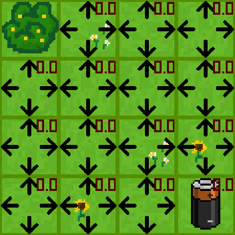
- Terminal state: If the robot hits the battery, it receives \(r=1\) (potentially discounted) and the episode ends.
- Optimal strategy: Move towards the battery as quickly as possible.
If we know the model (i.e., \(p\)), we can use the iterative policy evaluation algorithm:

Example: Gridworld
Now: Every-visit MC prediction of \(V^\pi\), for \(\policy{\cdot}{s} = [0.25, 0.25, 0.25, 0.25]^\top ~\forall~ s\in\Sc\).
Monte Carlo estimation of action values
Monte Carlo estimation of action values
Is a model available (i.e., the MDP \((\Sc, \Ac, p, r, \gamma)\) is known)?
- Yes \(\Rightarrow\) state values plus one-step predictions deliver an optimal policy.
- No \(\Rightarrow\) action values are very useful to directly obtain optimal policies.
Estimating \(Q^\pi(s,a)\) using MC:
- Analog to the MC prediction algorithm for \(V^\pi(s)\).
- Small variation: A visit refers to a state-action pair \((s,a)\).
- First-visit and every-visit variants exist
Possible challenges?
- Certain state-action pairs \((s,a)\) may never be visited.
- Missing degree of exploration (in particular for deterministic \(\pi\)).
- Workaraound: exploring starts \(\Rightarrow\) start episodes in random state-action pairs \((s,a)\).
Monte Carlo control
Monte Carlo control (1)
We learned about the Generalized policy iteration (GPI) in the last lecture.
Let’s use the same procedure here: \[ \pi_0 \stackrel{E}{\longrightarrow} Q^{\pi_0} \stackrel{I}{\longrightarrow} \pi_1 \stackrel{E}{\longrightarrow} Q^{\pi_1} \ldots \stackrel{I}{\longrightarrow} \pi^* \stackrel{E}{\longrightarrow} Q^*=Q^{\pi^*}. \]
Policy improvement: Make the policy greedy w.r.t. the current value function:
Since we have the action-value function \(Q\), we don’t need a model to construct the policy: \[ \pi(s) = \arg\max_{a\in\Ac} Q(s,a). \]


Monte Carlo control (2)
Even if we’re operating in an unknown MDP, the policy improvement theorem remains valid for MC-based control due to the underlying MDP structure:
Policy improvement theorem for MC-based control \[ \begin{align*} Q^{\pi_k}(s,\pi_{k+1}(s)) &= Q^{\pi_k}\left(s,\arg\max_{a\in\Ac} Q^{\pi_k}(s,a)\right) \\ &=\max_{a\in\Ac} Q^{\pi_k}(s,a) \\ &\geq Q^{\pi_k}(s,\pi_k(s)) \\ &\geq V^{\pi_k}(s). \end{align*} \]
- Policy improvement: Construct the greedy policy \(\pi_{k+1}(s)\) w.r.t. the current approximation \(Q^{\pi_k}\)
- Assumptions required:
- The episodes have epxloring starts. \(\qquad\qquad\qquad\qquad\) (We will consider this later)
- We are training on an infinite number of episodes.
Monte Carlo control (3)
Algorithm: Monte Carlo ES (Exploring Starts) for estimating \(\pi \approx \pi^*\).
initialize
- \(\pi(s)\) arbitrarily for \(s \in \Sc\)
- \(Q(s,a)\) arbitrarily for \(s \in \Sc\), \(a\in\Ac\)
- \(\ell(s,a)\): an empty list of returns for all \(s \in \Sc\), \(a\in\Ac\)
for \(k = 1, 2, \ldots, K\) episodes (or until \(\pi\) converges):
\(\quad\) \(g \gets 0\)
\(\quad\) Choose \(s_0\in\Sc\) and \(a_0\in\Ac\) randomly such that all pairs have probability \(>0\)
\(\quad\) Generate a sequence starting at \((s_0, a_0)\) and following \(\pi\): \[((s_0,a_0,r_0),(s_1,a_1,r_1),\ldots,(s_{T_k-1},a_{T_k-1},r_{T_k-1}))\] \(\quad\) for \(t = T_k-1,T_k-2,T_k-3,\ldots,0\):
\(\quad\quad\) \(g \gets \gamma g+ r_t\)
\(\quad\quad\) if \((s_t,a_t) \notin \{(s_0,a_0),\ldots,(s_{t-1},a_{t-1})\}\) then
\(\quad\quad\quad\) Append \(g\) to \(\ell(s_t)\)
\(\quad\quad\quad\) \(Q(s_t,a_t) = \mathsf{average}(\ell(s_t,a_t))\)
\(\quad\quad\quad\) \(\pi(s_t) \gets \arg\max_{a\in\Ac}Q(s_t, a)\)
- It is clear that this algorithm cannot converge to a suboptimal policy
- Stability is only achieved when both \(\pi\) and \(Q\) are optimal
Incremental implementation
- The previous algorithm (as well as all other before where we have used averaging) is computationally inefficient!
- Instead, it is better to update the estimate for \(Q\) (or \(V\)) incrementally.
- The sample mean \(\mu_1, \mu_2, \ldots\) of an arbitrary sequence \(g_1, g_2, \ldots\) is: \[ \mu_K = \frac{1}{K}\sum_{k=1}^K g_k \fragment{= \frac{1}{K} \left[g_K + \sum_{k=1}^{K-1} g_k\right]} \fragment{= \frac{1}{K} \left[g_K + (K-1)\mu_{K-1}\right]} \fragment{= \mu_{K-1} + \frac{1}{K} \left[g_K -\mu_{K-1}\right].} \]
- In terms of the averaging function from the algorithm before, this means that we can update \(Q(s_t,a_t)\) incrementally (with \(n(s_t,a_t)\) being the number of occurrences of the tuple \((s_t,a_t)\)): \[ Q(s_t,a_t) = \mathsf{average}(\ell(s_t,a_t)) \qquad\Rightarrow\qquad Q(s_t,a_t) \gets Q(s_t,a_t) + \frac{1}{n(s_t,a_t)} \left[g - Q(s_t,a_t)\right]. \]
💡 if a problem is non-stationary, we can use a step size \(\alpha\in(0,1]\) as in the multi-armed bandit setting: \(Q(s_t,a_t) = Q(s_t,a_t) + \alpha \left[g - Q(s_t,a_t)\right]\).
Monte Carlo control (4) – incremental implementation
Algorithm: Monte Carlo ES (Exploring Starts) for estimating \(\pi \approx \pi^*\).
initialize
- \(\pi(s)\) arbitrarily for \(s \in \Sc\)
- \(Q(s,a)\) arbitrarily for \(s \in \Sc\), \(a\in\Ac\)
- \(n(s,a)=0 ~ \forall ~ s \in \Sc\), \(a\in\Ac\): a list of state-action visits \(\qquad\)(
an empty list of returns \(\ell\))
for \(k = 1, 2, \ldots, K\) episodes (or until \(\pi\) converges):
\(\quad\) \(g \gets 0\)
\(\quad\) Choose \(s_0\in\Sc\) and \(a_0\in\Ac\) randomly such that all pairs have probability \(>0\)
\(\quad\) Generate a sequence starting at \((s_0, a_0)\) and following \(\pi\): \[((s_0,a_0,r_0),(s_1,a_1,r_1),\ldots,(s_{T_k-1},a_{T_k-1},r_{T_k-1}))\] \(\quad\) for \(t = T_k-1,T_k-2,T_k-3,\ldots,0\):
\(\quad\quad\) \(g \gets \gamma g + r_t\)
\(\quad\quad\) if \((s_t,a_t) \notin \{(s_0,a_0),\ldots,(s_{t-1},a_{t-1})\}\) then
\(\quad\quad\quad\) \(n(s_t,a_t) \gets n(s_t,a_t) + 1\) \(\qquad\qquad\qquad\qquad\qquad\qquad\qquad\) (appending \(g\) to the list of returns)
\(\quad\quad\quad\) \(Q(s_t,a_t) \gets Q(s_t,a_t) + \frac{1}{n(s_t,a_t)} \left[g - Q(s_t,a_t)\right]\)\(\qquad\quad\) (averaging over the list of returns )
\(\quad\quad\quad\) \(\pi(s_t) = \arg\max_{a\in\Ac}Q(s_t, a)\)
Example: Gridworld
Let’s apply the Monte Carlo Exploring Starts algorithm to two gridworlds of different sizes:
On-policy and off-policy learning
On-policy versus off-policy (1)
On-Policy: “Learning by Doing”
- The agent only learns from what it’s currently doing.
- It evaluates and improves the exact same policy it is using to make decisions.
- For example,
- if it is being cautious, it learns how to improve cautious behavior.
- if it tries something risky and fails, it learns from that failure but can’t easily “imagine” what would have happened if it had taken a different action earlier.
Off-Policy: “Learning by Observing”
- is more like a student watching an expert or looking at a variety of different actors once.
- It can follow one path (the “behavior policy”) while learning the best possible path (the “target policy”).
- It separates “how I am acting” from “what I am learning.”
- Benefit: It can learn from old data, from human demonstrations, or by watching other agents.
Question: Which class does the Monte Carlo ES algorithm belong to?
Answer: It is on-policy! Each time we update our policy (the counter \(k\) for the episodes), we collect the returns anew, following the current policy \(\pi\).
We will cover the topic on-policy versus off-policy in more detail later in this course.
On-policy versus off-policy (2)
| Feature | On-policy | Off-policy |
|---|---|---|
| Learning Source | Learns from its current actions only. | Can learn from any data (past, random, or expert). |
| Exploration | Often more stable but can get stuck in “safe” habits. | More aggressive at finding the absolute best strategy. |
| Efficiency | Lower. Throws away data once the policy changes. | Higher. Can “re-use” old experiences (Experience Replay). |
\(\epsilon\)-greedy as an on-policy alternative (1)
Motivating question: How do we get rid of the restrictive (and often not achievable) requirement of exploring starts (ES)?
- We need to make sure that we visit all state-action pairs, irrespective of where we start!
- Exploration requirement: \[ \pias > 0 \quad \forall s\in\Sc,a\in\Ac. \]
- Policies of this type are called soft.
- The level of exploration should be tunable during the learning process.
Where have we seen something like this before? \(\Rightarrow\) In the multi-armed bandits lecture!
\(\epsilon\)-greedy on-policy learning
- With probability \(\epsilon\), the agent’s choice (i.e., the policy output) is overwritten by a random action.
- Probability of all non-greedy actions: \(\frac{\epsilon}{\abs{\Ac}}\).
- Probability of the greedy action: \(1 - \epsilon + \frac{\epsilon}{\abs{\Ac}}\).
\(\epsilon\)-greedy as an on-policy alternative (2)
Algorithm: \(\epsilon\)-greedy on-policy first-visit MC control.
initialize
- \(\pi(s)\) arbitrarily for \(s \in \Sc\)
- \(Q(s,a)\) arbitrarily for \(s \in \Sc\), \(a\in\Ac\)
- \(n(s,a)=0 ~ \forall ~ s \in \Sc\), \(a\in\Ac\): a list of state-action visits
for \(k = 1, 2, \ldots, K\) episodes (or until \(\pi\) converges):
\(\quad\) \(g \gets 0\)
\(\quad\) Choose \(s_0\in\Sc\) and \(a_0\in\Ac\) randomly such that all pairs have probability \(>0\)
\(\quad\) Generate a sequence \(\set{(s_t,a_t,r_t)}_{t=1}^{T_k}\) starting at \((s_0, a_0)\) and following \(\pi\)
\(\quad\) for \(t = T_k-1,T_k-2,T_k-3,\ldots,0\):
\(\quad\quad\) \(g \gets \gamma g + r_t\)
\(\quad\quad\) if \((s_t,a_t) \notin \{(s_0,a_0),\ldots,(s_{t-1},a_{t-1})\}\) then
\(\quad\quad\quad\) \(n(s_t,a_t) \gets n(s_t,a_t) + 1\)
\(\quad\quad\quad\) \(Q(s_t,a_t) \gets Q(s_t,a_t) + \frac{1}{n(s_t,a_t)} \left[g - Q(s_t,a_t)\right]\)
\(\quad\quad\quad\) \(\tilde a = \arg\max_{a\in\Ac}Q(s_t, a)\)
\(\quad\quad\quad\) \(\policy{a}{s_t} = \begin{cases} 1-\epsilon+\epsilon/\abs{\Ac}, & a = \tilde{a} \\ \epsilon/\abs{\Ac}, & a \neq \tilde{a} \end{cases}\)
\(\epsilon\)-greedy policy improvement
Theorem: Policy improvement for \(\epsilon\)-greedy policies
Given an MDP, an \(\epsilon\)-greedy policy \(\pi'\) w.r.t. \(Q^\pi\) is an improvemnt over the \(\epsilon\)-soft policy \(\pi\), i.e., \(V^{\pi^\prime} > V^\pi\) for all \(s\in\Sc\).
Proof: \[ \begin{align*} V^{\pi^\prime}(s)=Q^\pi(s,\pi'(s)) &= \sum_{a\in\Ac} \pi'\agivenb{a}{s} Q^\pi(s,a) \\ &= \frac{\epsilon}{\abs{\Ac}}\left(\sum_{a\in\Ac} Q^\pi(s,a)\right) + (1-\epsilon) \max_{a\in\Ac} Q^\pi(s,a)\\ &\geq \frac{\epsilon}{\abs{\Ac}}\left(\sum_{a\in\Ac} Q^\pi(s,a)\right) + (1-\epsilon) \left( \sum_{a\in\Ac} \frac{\pias-\frac{\epsilon}{\abs{\Ac}}}{1-\epsilon} Q^\pi(s,a)\right)\\ \textit{(Last term: weighted }&\text{average over all actions. It thus has to be smaller than the max operation.)}\\ &=\frac{\epsilon}{\abs{\Ac}}\left(\sum_{a\in\Ac} Q^\pi(s,a)\right) - \frac{\epsilon}{\abs{\Ac}}\left(\sum_{a\in\Ac} Q^\pi(s,a)\right) + \sum_{a\in\Ac} \pias Q^\pi(s,a)\\ &= V^\pi(s). \end{align*} \]
Greedy in the limit with infinite exploration (GLIE)
Definition: Greedy in the limit with infinite exploration (GLIE)
A learning policy \(\pi\) is called GLIE if it satisfies the following two properties:
- If a state is visited infinitely often, then each action is chosen infinitely often: \[ \lim_{k\rightarrow\infty} \pi_k\agivenb{a}{s} = 1 \quad \forall~s\in\Sc,a\in\Ac. \]
- In the limit (\(i\rightarrow\infty\)) the learning policy is greedy with respect to the learned action value: \[ \lim_{k\rightarrow\infty} \pi_k\agivenb{a}{s} = \pi(s) = \arg\max_{a\in\Ac} Q^\pi(s,a)\quad \forall s\in\Sc. \]
GLIE Monte Carlo control
Theorem: Optimal decision using MC-control with \(\epsilon\)-greedy
MC-based control using \(\epsilon\)-greedy exploration is GLIE, if \(\epsilon\) is decreased at rate \[ \epsilon_k=\frac{1}{k}, \] with \(k\) being the increasing episode index. In this case, \[ Q^\pi(s,a)=Q^*(s,a). \]
Remarks:
- Limited feasibility: infinite number of episodes required.
- \(\epsilon\)-greedy is an undirected and unmonitored random exploration strategy. Can that be the most efficient way of learning?
Example: Gridworld - fixed starting point
Fixed-start, every-visit action-value estimation:
Example: Gridworld - exploring starts
Exploting starts (ES), every-visit action-value estimation:
Off-policy Monte Carlo control
Off-policy learning background
All learning control methods face a dilemma:
- They seek to learn action values conditional on subsequent optimal behavior,
- but they need to behave non-optimally in order to explore all actions.
- The previous \(\epsilon\)-greedy approaches were only a compromise: learning action values for near-optimal policies.
The off-policy learning idea:
- Use two policies:
- Behavior policy \(\pi_\beta\agivenb{a}{s}\): exploratory, used to generate behavior.
- Target policy \(\pias\): learns from that experience to become the optimal policy.
- Use cases:
- Learn from observing humans or other agents/controllers.
- Re-use experience generated from old policies (\(\pi_0,\pi_1,\ldots\)).
- Learn about multiple policies while following one policy.
Off-policy prediction problem statement
MC off-policy prediction problem statement.
- Both policies are considered fixed (that’s the prediction assumption).
- Estimate \(V^\pi\) or \(Q^\pi\) while following \(\pi_\beta\agivenb{a}{s}\).
Requirement:
- Coverage: every action taken under \(\pi\) must be (at least occasionally) taken under \(\pi_\beta\) as well. \[ \pias > 0 \quad\Rightarrow\quad \pi_\beta\agivenb{a}{s}>0 \qquad \forall s\in\Sc, a\in\Ac. \]
- Consequence:
- In any state where \(\pi_\beta\neq \pi\), \(\pi_\beta\) has to be a stochastic policy.
- Nevertheless, \(\pi\) may be either stochastic or deterministic.
Importance sampling (1)
Example
- We’re trying to calculate the average height of people in a city, but only have access to a guest list for a professional basketball convention.
- Taking the average of this sample will likely lead to a too large value.
- Importance sampling: mathematical correction to use data from one distribution to estimate properties of another distribution.

The central concept: re-weighting
- We want to know the expected value under a target distribution \(\pi(s)\), but only have samples from another distribution \(\pi_\beta(s)\).
- We calculate the importance weight: \[w = \frac{\pi(s)}{\pi_\beta(s)}\]
- If a sample is common in \(\pi\) but rare in \(\pi_\beta\), we give it a high weight (it is important).
- If a sample is rare in \(\pi\) but common in \(\pi_\beta\), we give it a low weight.
Caveat: if \(w\) is large (distinctly different policies) the estimate’s variance is large (i.e., uncertain for small numbers of samples).
Importance sampling (2)
Given a starting state \(s_t\), the probability of the subsequent state–action trajectory \((a_t, s_{t+1},a_{t+1}, \ldots ,s_T)\) under a policy \(\pi\) is \[ \begin{align*} \pC{a_t, s_{t+1},a_{t+1}, \ldots ,s_T}{s_t,\pi} &= \policy{a_t}{s_t}\pC{s_{t+1}}{s_t,a_t}\fragment{\policy{a_{t+1}}{s_{t+1}}\pC{s_{t+2}}{s_{t+1},a_{t+1}}}\fragment{\ldots \pC{s_{T}}{s_{T-1},a_{T-1}}}\\ &= \prod_{k=t}^{T-1} \policy{a_k}{s_k}\pC{s_{k+1}}{s_{k},a_{k}}. \end{align*} \]
Importance sampling ratio
The relative probability of a trajectory under the target and behavior policy, the importance sampling ratio, from sample step \(k\) to \(T\) is \[ \rho_{t:T} = \frac{\prod_{k=t}^{T-1} \policy{a_k}{s_k}\pC{s_{k+1}}{s_{k},a_{k}}}{\prod_{k=t}^{T-1} \pi_\beta\agivenb{a_k}{s_k}\pC{s_{k+1}}{s_{k},a_{k}}} \fragment{= \frac{\prod_{k=t}^{T-1} \policy{a_k}{s_k}\cancel{\pC{s_{k+1}}{s_{k},a_{k}}}}{\prod_{k=t}^{T-1} \pi_\beta\agivenb{a_k}{s_k}\cancel{\pC{s_{k+1}}{s_{k},a_{k}}}}} \fragment{= \frac{\prod_{k=t}^{T-1} \policy{a_k}{s_k}}{\prod_{k=t}^{T-1} \pi_\beta\agivenb{a_k}{s_k}}.} \]
💡 Although the trajectory probabilities depend on the MDP’s transition probabilities \(p\) (which are generally unknown), the importance sampling ratio ends up depending only on the two policies and the sequence, not on the MDP.
Importance sampling for MC prediction
- We wish to estimate the expected returns \(g_t\) under the target policy \(\pi\), but we only have \(g_t\) due to the behavior policy \(\pi_\beta\).
- These returns have the wrong expectation: \[\ExpC{g_t}{s_t=s} = V^\beta(s).\]
- Importance sampling: \[\ExpC{\rho_{k:T}\, g_t}{s_t=s} = V^\pi(s).\]
OIS: State-value estimation via Monte Carlo ordinary importance sampling
Estimating the state value \(V^\pi\) following a behavior policy \(b\) using ordinary importance sampling (OIS) results in scaling and averaging the sampled returns by the importance sampling ratio per episode: \[ \begin{equation} V^\pi(s) = \frac{\sum_{t\in\mathcal{T}(s)}\rho_{k:T(t)}\, g_t}{\abs{\mathcal{T}(s)}}. \tag{OIS} \label{eq:MC_OIS} \end{equation} \] Here \(\mathcal{T}(s)\) is the set of all time steps in which \(s\) is visited, and \(T(t)\) is the termination of the episode starting at \(t\).
Weighted importance sampling
- OIS can be shown to be unbiased (Sutton and Barto 1998), meaning that the expectation of \(\eqref{eq:MC_OIS}\) is always \(V^\pi\).
- On the other hand, it can be extreme.
WIS: State-value estimation via Monte Carlo importance sampling
Estimating the state value \(V^\pi\) following \(\pi_\beta\) using weighted importance sampling (WIS) results in a slightly different scaling: \[ \begin{equation} V^\pi(s) = \frac{\sum_{t\in\mathcal{T}(s)}\rho_{k:T(t)}\, g_t}{\sum_{t\in\mathcal{T}(s)}\rho_{k:T(t)}}. \tag{WIS} \label{eq:MC_WIS} \end{equation} \]
Main differences between the two (first-visit) versions:
- Bias:
- \(\eqref{eq:MC_OIS}\) is unbiased.
- \(\eqref{eq:MC_WIS}\) is biased (though it converges asymptotically to zero).
- Variance:
- The variance of \(\eqref{eq:MC_OIS}\) is in general unbounded (the variance of the ratios can be unbounded).
- For \(\eqref{eq:MC_WIS}\), the largest weight on any single return is one.
- Assuming bounded returns, the variance of \(\eqref{eq:MC_WIS}\) converges to zero even if the variance of the ratios themselves is infinite (Precup, Sutton, and Dasgupta 2001)
- In practice, \(\eqref{eq:MC_WIS}\) has dramatically lower variance and is strongly preferred.
WIS: incremental implementation
If we want to perform weighted importance sampling in an in an incremental fashion, we need to keep track of all the weights in \(\eqref{eq:MC_WIS}\). Let’s do this exemplary for the value function \(V_k\) at iteration \(k\): \[ V_k = \frac{\sum_{t=1}^{n} w_t g_t}{\sum_{t=1}^{n} w_t}, \qquad \text{where}\quad w_t=\rho_{k:T(t)}. \] In addition to keeping track of \(V_k\), we must maintain for each state the cumulative sum \(c_k\) of the weights given to the first \(k\) returns. The update rule for \(V_k\) is then: \[ V_{k+1} = V_k + \frac{w_k}{c_k}\left[g_k - V_k\right] \qquad \fragment{\text{and} \qquad c_{k+1} = c_k + w_{k+1},} \] with \(c_0=0\).
Off-policy Monte Carlo control (1)
Algorithm: Off-policy MC prediction (policy evaluation) for \(Q\approx Q^*\).
initialize (for all \(s \in \Sc\), \(a\in\Ac\))
- \(Q(s,a)\) arbitrarily
- \(c(s,a) \gets 0\)
for \(k = 1, 2, \ldots, K\) episodes (or until \(\pi\) converges):
\(\quad\) \(g \gets 0\), \(w \gets 1\)
\(\quad\) Generate \(\set{(s_t,a_t,r_t)}_{t=0}^{T_k}\) following a soft policy \(b\)
\(\quad\) for \(t = T_k-1,T_k-2,T_k-3,\ldots,0\):
\(\quad\quad\) \(g \gets \gamma g + r_t\)
\(\quad\quad\) \(c(s_t,a_t) \gets c(s_t,a_t) + w\)
\(\quad\quad\) \(Q(s_t,a_t) \gets Q(s_t,a_t) + \frac{w}{c(s_t,a_t)} \left[g - Q(s_t,a_t)\right]\)
\(\quad\quad\) \(w \gets w \frac{\policy{a_t}{s_t}}{\pi_\beta\agivenb{a_t}{s_t}}\)
Variation: On-policy
- \(\pi_\beta=\pi\) .
- \(\frac{\policy{a_t}{s_t}}{\pi_\beta\agivenb{a_t}{s_t}}=1\).
- \(w=1\).
- \(c(s,a)\) becomves the counter for the number of visits (i.e., \(n(s,a)\)).
Off-policy Monte Carlo control (2)
We now have our final algorithm that includes everything we have learned so far
Algorithm: Off-policy MC control for estimating \(Q\approx Q^*\) and \(\pi\approx\pi^*\).
initialize (for all \(s \in \Sc\), \(a\in\Ac\))
- \(Q(s,a)\) arbitrarily
- \(c(s,a) \gets 0\)
- \(\pi(s)=\arg\max_{a\in\Ac}Q(s,a)\) (with ties broken consistently)
for \(k = 1, 2, \ldots, K\) episodes (or until \(\pi\) converges):
\(\quad\) \(g \gets 0\), \(w \gets 1\)
\(\quad\) Generate \(\set{(s_t,a_t,r_t)}_{t=0}^{T_k}\) following a soft policy \(b\)
\(\quad\) for \(t = T_k-1,T_k-2,T_k-3,\ldots,0\):
\(\quad\quad\) \(g = \gamma g + r_t\)
\(\quad\quad\) \(c(s_t,a_t) \gets c(s_t,a_t) + w\)
\(\quad\quad\) \(Q(s_t,a_t) \gets Q(s_t,a_t) + \frac{w}{c(s_t,a_t)} \left[g - Q(s_t,a_t)\right]\)
\(\quad\quad\) \(\pi(s_t) \gets \arg\max_{a\in\Ac}Q(s_t,a)\) (with ties broken consistently)
\(\quad\quad\) if \(\pi(s_t)\neq a_t\) then
\(\quad\quad\quad\) Exit inner loop and proceed to next episode
\(\quad\quad\) \(w \gets w \frac{1}{\pi_\beta\agivenb{a_t}{s_t}}\)
Summary / what you have learned
Summary / what you have learned
- MC methods allow model-free learning of value functions and optimal policies from experience (i.e., sampled episodes).
- Using full episodes, MC is largely based on averaging returns.
- MC-based control reuses generalized policy iteration (GPI), i.e., mixing policy evaluation and improvement.
- Maintaining sufficient exploration is important:
- Exploring starts: not feasible in all applications but simple.
- On-policy \(\epsilon\)-greedy learning: trade-off between exploitation and exploration cannot be resolved easily.
- Off-policy learning: agent learns about a (possibly deterministic) target policy from an exploratory, soft behavior policy.
- Importance sampling transforms expectations from the behavior to the target policy.
- This estimation task comes with a bias-variance-dilemma.
- Slow learning can result from ineffective experience usage in MC methods.
References
Precup, Doina, Richard S Sutton, and Sanjoy Dasgupta. 2001. “Off-Policy Temporal-Difference Learning with Function Approximation.” In ICML, 417–24.
Sutton, R. S., and A. G. Barto. 1998. Reinforcement Learning: An Introduction. MIT Press.