Content

Content:

The three main learning paradigms
Supervised learning
- The learning diagram
- Generalization
- Bias & variance
- Cross-validation
Deep neural networks
- Artificial neural networks
- Multi-layer perceptron
- Training
- Regularization
- Neural network architectures
Linear regression as a special case

Useful references:

Pattern recognition and machine learning (Bishop 2006)
Deep learning (Bengio et al. 2017)
The elements of statistical learning (Hastie 2009)
Learning from data: a short course (Abu-Mostafa, Magdon-Ismail, and Lin 2012)

Where are we?

Lecture contents
Chapter	Topic	Content
	Basics & tabular methods
1-5	Bandits, MDPs, Dynamic Programming, Monte Carlo, TD Learning	RL basics in finite dimensions
	Deep-learning-based methods
6	Brief introduction to deep learning	The basics for what comes next
7	Value function approximation
8	Deep $Q$-learning
9	Policy gradients
10	Actor-critic algorithms
11	Advanced algorithms (Part I): From policy gradient to PPO
12	Advanced algorithms (Part II): From $Q$-learning to Soft Actor-Critic
	Model-Based Control
	Advanced Topics

The three main learning paradigms

The three big learning paradigms (Abdelwanis et al. 2026) (Examples: Unsupervised, Supervised, RL)

Supervised learning

The learning diagram

The learning diagram (Abu-Mostafa, Magdon-Ismail, and Lin 2012)

Generalization

What does it mean to have a perfect model on your training dataset $\Dtrain$, i.e., $L(\theta; \Dtrain) = 0$?
$\Rightarrow$ we have simply memorized the data!
Learning means that we get good predictions on unseen data: \[ \underbrace{L(\theta; \Dtest)}_{\text{out-of-sample error}} \approx \underbrace{L(\theta; \Dtrain)}_{\text{in-sample error}}. \]

Supervised learning

Given a labeled (and probably noisy) dataset $\Dtrain=\{(x_1,y_1),\ldots,(x_N,y_N)\}$, approximate the unknown mapping $f : \Xc \to \Yc$ by a parametrizable ML model $f_\theta: \Xc \to \Yc$, such that \[ f_\theta(x_k) = \hat{y}_k \approx y_k \quad \forall ~ (x_k,y_k)\in\Dtest .\]

Goodness of fit can be measured via many different metrics (e.g., mean squared error, classification accuracy, etc.).
The dimension $d$ of model parameters $\theta \in\R^d$ is adjustable in many model families, which trades off bias with variance (among other factors, leading to so-called under- and overfitting).
On top of $\theta$, an ML model might also have hyperparameters that can be optimized (e.g., number of layers in a neural network).

Bias-variance tradeoff (1)

$\bullet$ In the ML context, bias denotes the error of the average model $\overline{f}_{\theta}$ when repeating the training with different datasets $\Dc_{\mathsf{train},1},\Dc_{\mathsf{train},2},\ldots$: \[ \mathsf{bias} = \Expsub{\left(\overline{f}_{\theta}(x) - f(x)\right)^2}{x\sim\Dtest}. \]

$\bullet$ variance denotes the variability in between the individual training runs: \[ \mathsf{variance} = \Expsub{\Expsub{\left(f^{(\Dc)}_{\theta}(x) - \overline{f}_{\theta}(x)\right)^2}{\Dc\sim\{\Dc_{\mathsf{train,\ell}}\}_{\ell=1}^\infty}}{x\sim\Dtest}. \]

$\Rightarrow$ Often a matter of model complexity.

images/06-deep-learning/BV-En_low_bias_low_variance.png Low bias, low variance

images/06-deep-learning/BV-Truen_bad_prec_ok.png Large bias, low variance

images/06-deep-learning/BV-Truen_ok_prec_bad.png Low bias, large variance

images/06-deep-learning/BV-Truen_bad_prec_bad.png Large bias, large variance [Wikipedia]

Bias-variance tradeoff (2)

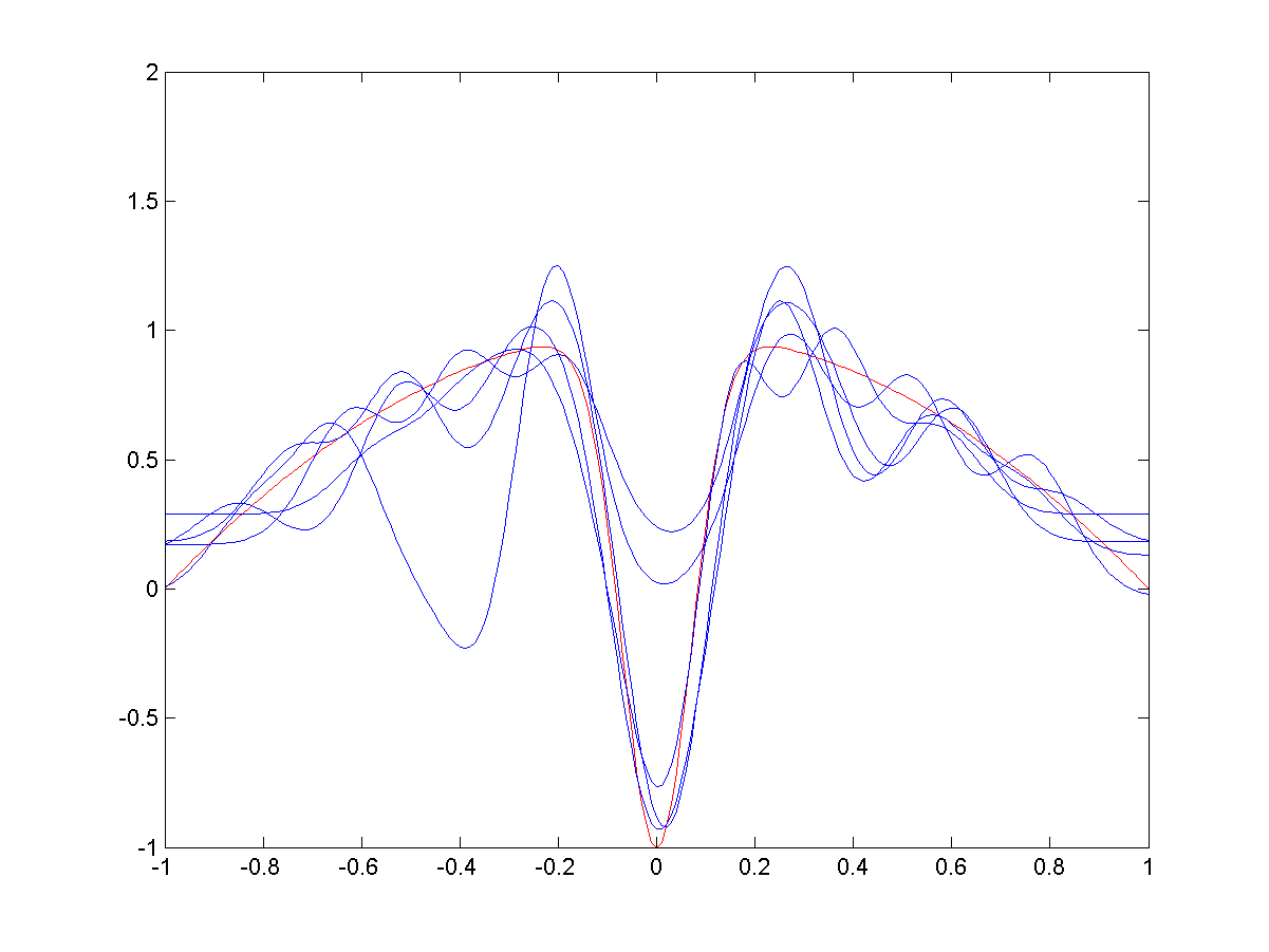
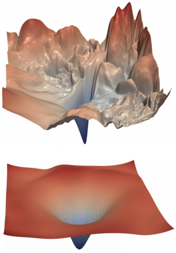
Example (see Wikipedia): Fitting a model of serveral radial basis functions to noisy trainig data: \[ f_\theta(x) = \sum_{k=1}^d \theta_k \exp\left(-\frac{1}{2}\frac{x-c_k}{\sigma_k^2}\right). \]

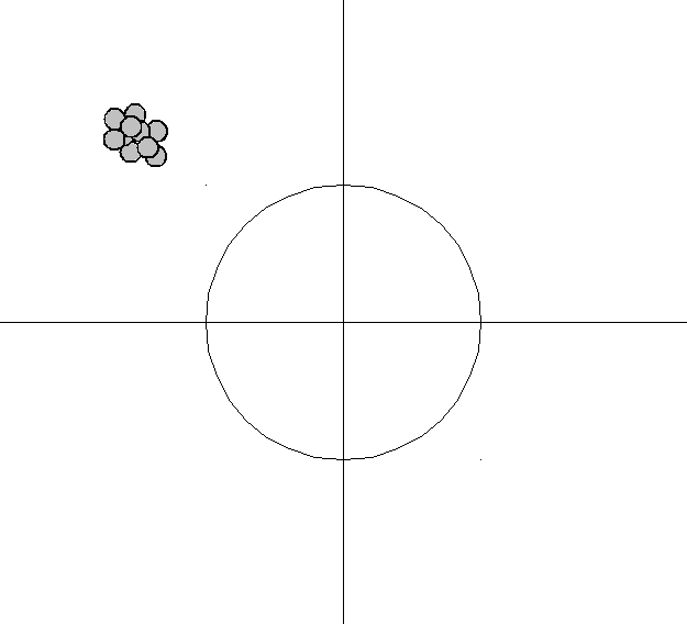
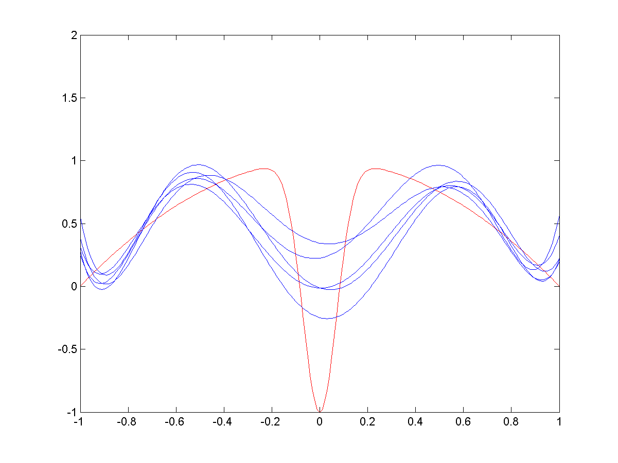
$\bullet$ For a wide spread (i.e., large $\sigma_k$), the bias is high: the RBFs cannot fully approximate the function (especially the central dip), but the variance between different trials is low.

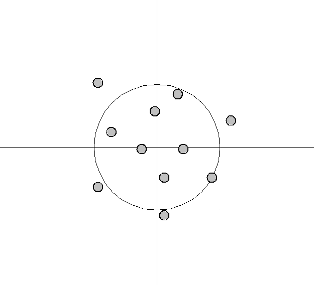
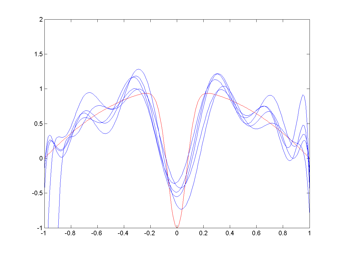
$\bullet$ As spread decreases (image 3 and 4) the bias decreases: the blue curves more closely approximate the red…

$\bullet$ … but the variance between trials ($\Dc_{\mathsf{train,1}},\Dc_{\mathsf{train,2}},\ldots$) increases.

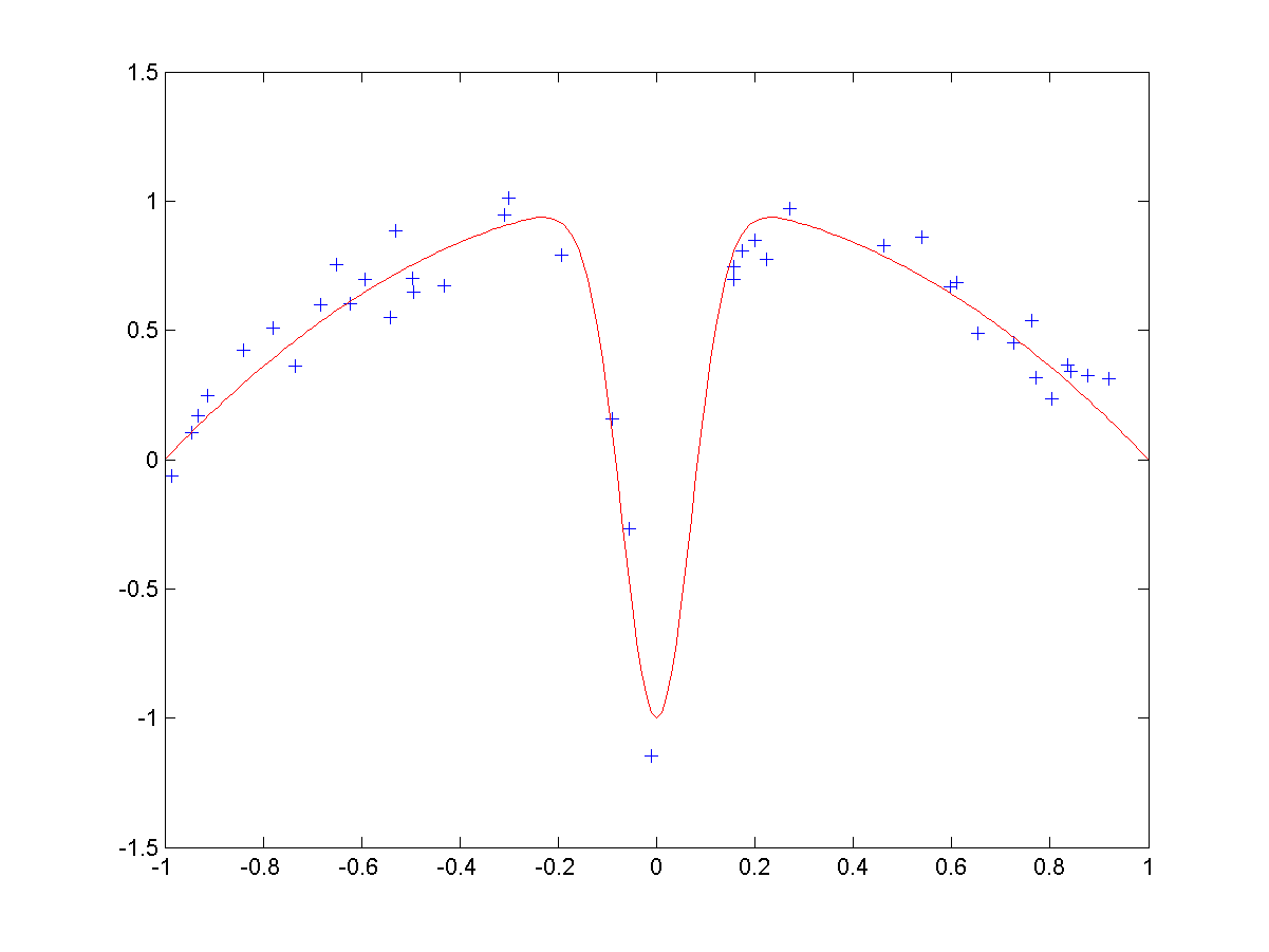
images/06-deep-learning/BV-Test_function_and_noisy_data.png — Function and training data $\Dc_{\mathsf{train,1}}$.

images/06-deep-learning/BV-Radial_basis_function_fit,_spread=5.png Wide spread RBFs.

images/06-deep-learning/BV-Radial_basis_function_fit,_spread=1.png Medium spread RBFs.

images/06-deep-learning/BV-Radial_basis_function_fit,_spread=0.1.png Small spread RBFs.

Cross-validation

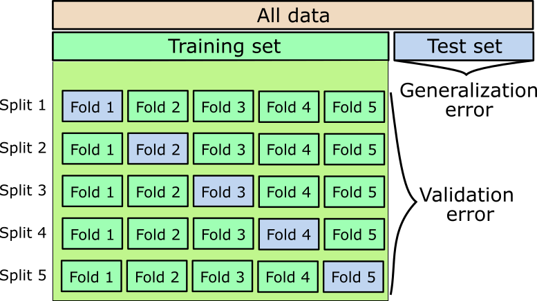
Training is repeated $k$ times with $k$ different splits of the training set.
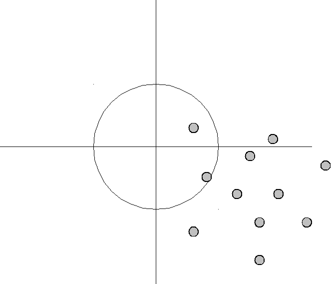
Each observation serves as unseen instance (blue boxes) at least once.
The validation error is an indicator for tuning hyperparameters.
Example of a $k$-fold Cross-validation (CV).

Means to improve a supervised learning model

Collecting more data, i.e., increasing $N$.
Reducing noise in the data.
Improving the distribution within the dataset, i.e., ensuring that the data set is representative of the problem domain.
Choosing a more appropriate model. A genereal rule is to select the model according to the amount of data one has, not according to the expected complexity of the funtion to approximate.
Optimizing hyperparameters of the model.
Ensemble learning: Averaging over several different models.
Including knowledge, e.g., in the form of tailored features (feature engineering) or informed loss functions.
- This is known as inductive bias in the ML literature.

Euclidean vs. polar coordinates/features in binary classification (Abdelwanis et al. 2026).

Deep neural networks

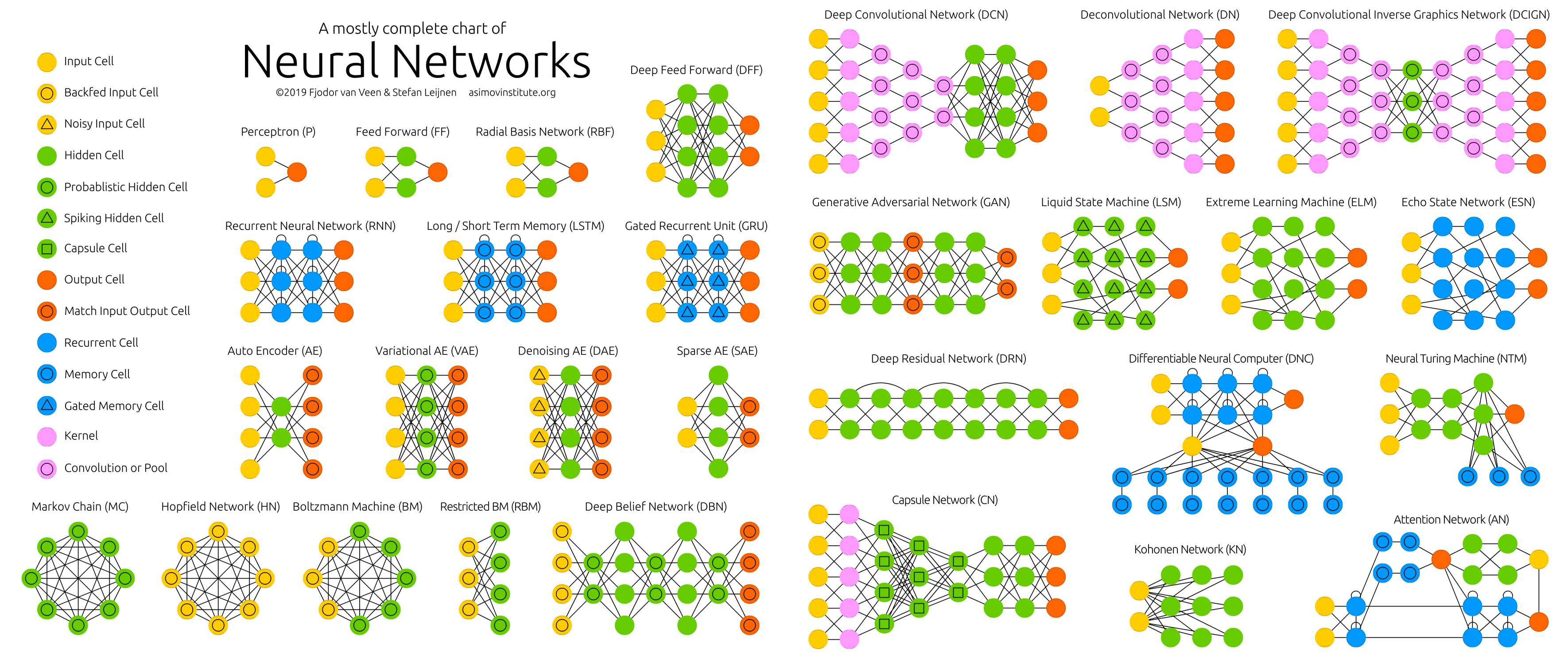
Artificial neural networks

Artificial neural networks (ANNs) are nonlinear function approximators $\hat{y}=f_\theta(x)$ that

are end-to-end differentiable.
are stacks of minimal units, the artificial neurons.

images/06-deep-learning/neuron.svg — An artificial neuron (Abdelwanis et al. 2026).

An ANN consists of nodes or neurons in one or more layers.
Each node transforms the weighted sum of all previous nodes (plus a potential bias term) through an activation function $\sigma$: \[ \sigma\left( \theta_0 + \sum_{k=1}^n \theta_k x_k \right). \]
The weighted connections are called edges, which represent the ANN’s parameters.

Multi-layer perceptron

Standard model of supervised learning: multi-layer perceptron or feed-forward ANN.

images/06-deep-learning/MLP.svg — MLP architecture (Abdelwanis et al. 2026).

Only forward-flowing edges.
The depth $L$ and width $\iterate{H}{\ell}$ are hyperparameters.
With $\iterate{\sigma}{\ell}$ and $\iterate{z}{\ell}$ denoting the activation function and activation of layer $\ell$ respectively, we get for the output in the $\th{\ell}$ layer. \[ \iterate{x}{\ell}= \iterate{\sigma}{\ell}\big( \underbrace{\iterate{\Theta}{\ell}\iterate{x}{\ell-1} + \iterate{b}{\ell}}_{\iterate{z}{\ell}} \big) ,\] with input $\iterate{x}{0}=x$ and output $\iterate{x}{L}=y$:
Training:
- Summarize the full set of parameters (i.e., weight matrices $\iterate{\Theta}{\ell}\in\R^{\iterate{H}{\ell} \times \iterate{H}{\ell-1}}$ and biases $\iterate{b}{\ell}$) under $\theta$.
- Iteratively update the weights using gradient information.

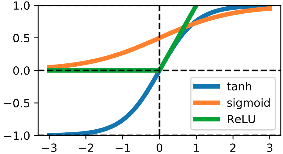
Activation functions

The source of nonlinearity in neural networks.$^*$
Common choices for $\sigma(z)$ are
- $\sigma(z) = \tanh(z)$,
- Sigmoid: $\sigma(z) = \frac{1}{1+e^{-z}}$,
- Rectified linear unit (ReLU): $\sigma(z) = \max(0, z)$,

images/06-deep-learning/activation.png — Exemplary activation functions (Abdelwanis et al. 2026).

The activation of the output layer, $\iterate{\sigma}{L}(z)$, is task-dependent. For instance,
- regression: $y=\iterate{\sigma}{L}(\iterate{z}{L})=\iterate{z}{L}$, i.e., $\iterate{\sigma}{L} = \mathsf{Id}$ is the identity mapping.
- binary classification: sigmoid (i.e., probability), followed by a rounding step to either $0$ or $1$.
- multi-class classification: $y_i=\frac{\exp(\iterate{z}{L}_i)}{\sum_j \exp(\iterate{z}{L}_j)}$ (softmax).

Training (1)

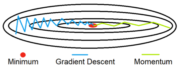
Training is performed in an iterative manner: \[\theta \gets \theta + \eta \delta\theta.\]
- $\eta\in\R_{>0}$ is the step size or learning rate.
- $\delta\theta\in\R^d$ is the update direction, usually a gradient-based descent direction.
- Numerous variants for $\delta\theta$. The strongest contain additional momentum terms such as the Adam algorithm (Kingma and Ba 2014). We remember the previous update $\delta\theta^{-}$ and thereby flatten out zig-zag behavior.
  Source
First, we need to define a loss function that we wish to minimize.
- Regression: (root) mean square error, mean absolute error.
- Classification: cross entropy.
- Additional terms, e.g., regularization, physics information, …
Iterations over the dataset $\Dtrain$ are called epochs.

images/06-deep-learning/loss-landscapes.png — The loss landscape of deep neural networks (with and without skip-connection) (Li et al. 2018).

Training (2)

The descent direction is computed by taking the derivative of the loss function w.r.t. the weight vector. In terms of the MSE: \[\begin{align*} \nabla L(\theta) &= \nabla \left(\frac{1}{N} \sum_{k=1}^N \norm{f_\theta(x_k) - y_k}_2^2 \right) \\ &= \frac{1}{N} \sum_{k=1}^N \nabla \norm{f_\theta(x_k) - y_k}_2^2 \qquad &&\text{(Linearity of the sum)}\\ &= \frac{1}{N} \sum_{k=1}^N \left(2 \cbracket{f_\theta(x_k) - y_k} \nabla f_\theta(x_k)\right) &&\text{(Chain rule of differentiation)} \end{align*}\]
This means that we need to propagate the error through our model $f_\theta$.
Since a neural network is a chain of neurons, we need to apply the chain rule of differentiation over the layers.
As a consequence the loss is backpropgated through the network to determine the individual descent directions: $\pdiff{L}{\theta_i}$.

This is called the backpropagation algorithm. We require one forward pass and one backward pass for every data tuple $(x_k,y_k)$. Taking the average gives us the average steepest-descent improvement over the dataset $\Dtrain$ for the current $\theta$.

Backpropagation example

Let’s consider a very simple network with $x,y\in\R$ and two hidden layers with a single neuron each.

Symbolic

\[ \stackrel{x}{\bigcirc} \underbrace{ \underbrace{\stackrel{\theta_1}{\longrightarrow} \stackrel{\iterate{z}{1}}{\bigcirc} \stackrel{\sigma}{\longrightarrow}}_{\text{Hidden\\ Layer}~1} \stackrel{\iterate{x}{1}}{\bigcirc} \underbrace{\stackrel{\theta_2}{\longrightarrow} \stackrel{\iterate{z}{2}}{\bigcirc} \stackrel{\sigma}{\longrightarrow}}_{\text{Hidden\\ Layer}~2} \stackrel{\iterate{x}{2}}{\bigcirc} \underbrace{\stackrel{\theta_3}{\longrightarrow}}_{\text{Output\\ layer}} }_{\hat{y}=f_\theta(x)} \stackrel{\hat{y}}{\bigcirc} \stackrel{L}{\longrightarrow} \stackrel{\text{Loss}}{\bigcirc} \]

$\quad$In mathematical terms

\[\begin{align*} \hat{y} &= \theta_3 \big( \iterate{x}{2} \big) \fragment{= \theta_3 \big( \sigma \big( \iterate{z}{2} \big) \big)} \fragment{= \theta_3 \big( \sigma \big( \theta_2 \big( \iterate{x}{1} \big) \big) \big)} \\ &= \theta_3 \big( \sigma \big( \theta_2 \big( \theta\big(\iterate{z}{1}\big) \big) \big) \big) \fragment{= \theta_3 \underbrace{\sigma\big(\theta_2 \overbrace{\sigma\big( \theta_1 x \big)}^{\text{Hidden\\ Layer}~1} \big)}_{\text{Hidden\\ Layer}~2}} \end{align*}\]

Let’s assume a single sample $(x,y)$ and the MSE loss: $L(\theta)=(\hat{y}-y)^2$. Using the chain rule, we get:

$1.$ Gradient w.r.t. $\theta_3$: \[ \pdiff{L}{\theta_3} = \textcolor{red}{\underbrace{\pdiff{L}{\hat{y}}}_{=2(\hat{y}-y)}}\pdiff{\hat{y}}{\theta_3}. \]

$2.$ Gradient w.r.t. $\theta_2$: \[ \pdiff{L}{\theta_2} = \textcolor{red}{\pdiff{L}{\hat{y}}}\textcolor{blue}{\pdiff{\hat{y}}{\iterate{x}{2}}\underbrace{\pdiff{\iterate{x}{2}}{\iterate{z}{2}}}_{=\sigma'}}\pdiff{\iterate{z}{2}}{\theta_2}. \]

$3.$ Gradient w.r.t. $\theta_1$: \[ \pdiff{L}{\theta_1} = \textcolor{red}{\pdiff{L}{\hat{y}}}\textcolor{blue}{\pdiff{\hat{y}}{\iterate{x}{2}}\underbrace{\pdiff{\iterate{x}{2}}{\iterate{z}{2}}}_{=\sigma'}}\textcolor{green}{\pdiff{\iterate{z}{2}}{\iterate{x}{1}}\underbrace{\pdiff{\iterate{x}{1}}{\iterate{z}{1}}}_{=\sigma'}}\pdiff{\iterate{z}{1}}{\theta_1}. \]

$\Rightarrow$ we propagate the loss back through the network, reusing most of the previous calculations!

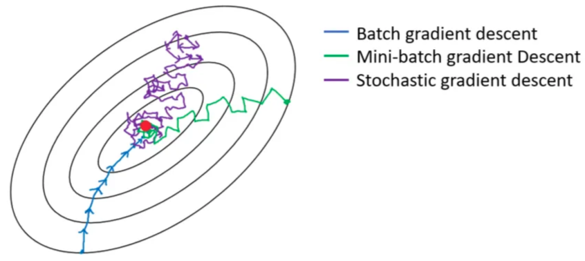
Stochastic gradient descent and batch learning

The cost for a single gradient step scales with the dataset size $N$, which can be very large.
For each sample, we need to perform one forward and one backward pass.
Stochastic gradient descent (SGD): massive speedup by using a single sample per step insetad of the entire dataset, \[\delta \theta = \nabla L(\theta; x_k), \qquad k\sim U(\{1,\ldots,N\}). \]
Mini-batch gradient descent with $s\in\{1,\ldots,N\}$ samples per step: compromise ground between efficiency and noisiness, \[ \delta \theta = \frac{1}{s} \sum_{k\in\mathcal{I}} \nabla L(\theta; x_k), \qquad \text{where}~\mathcal{I}~\text{is an $s$-dimensional, ranodmly drawn subset of $\{1,\ldots,N\}$}.\]

images/06-deep-learning/GD-SGD.png — Gradient descent vs. SGD vs. Mini-batch gradient descent [Sourcre].

Regularization

In order to mitigate overfitting (i.e., good performacne on $\Dtrain$, poor generalization), neural networks can be regularized by

Weight decay: adding an $\ell_2$ penalty term to the weights: $L(\theta) + \lambda \norm{\theta}_2^2$
Layer normalization during training: all layers’ activations are normalized separately by standard scaling,
Dropout: randomly disable nodes’ contribution.
- This helps especially in deep networks,
- and effectively builds an ensemble of ANNs with shared edges.

Convolutional neural networks

In machine learning (as well as in nature) many tasks are independent of absolute position.

A function is invariant under some transformation if it’s output $y$ remains unchanged under transformations of the input $x$.

A function is equivariant under some transformation if it’s output $y$ is transformed “in the same way” as the input $x$.

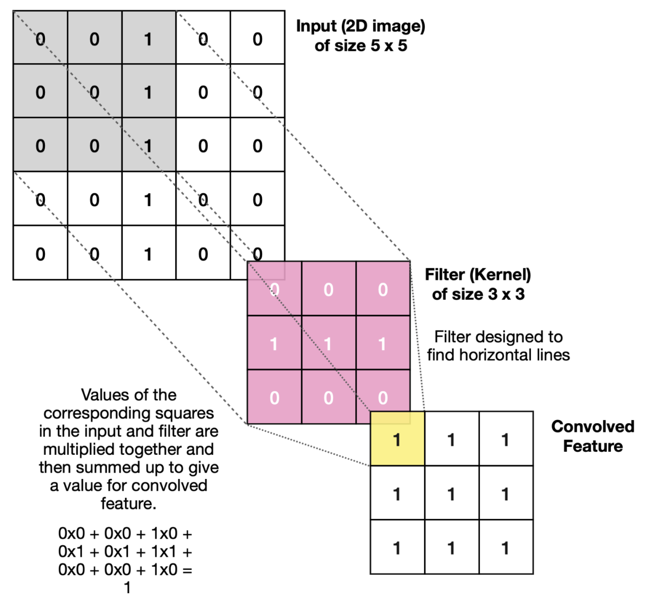
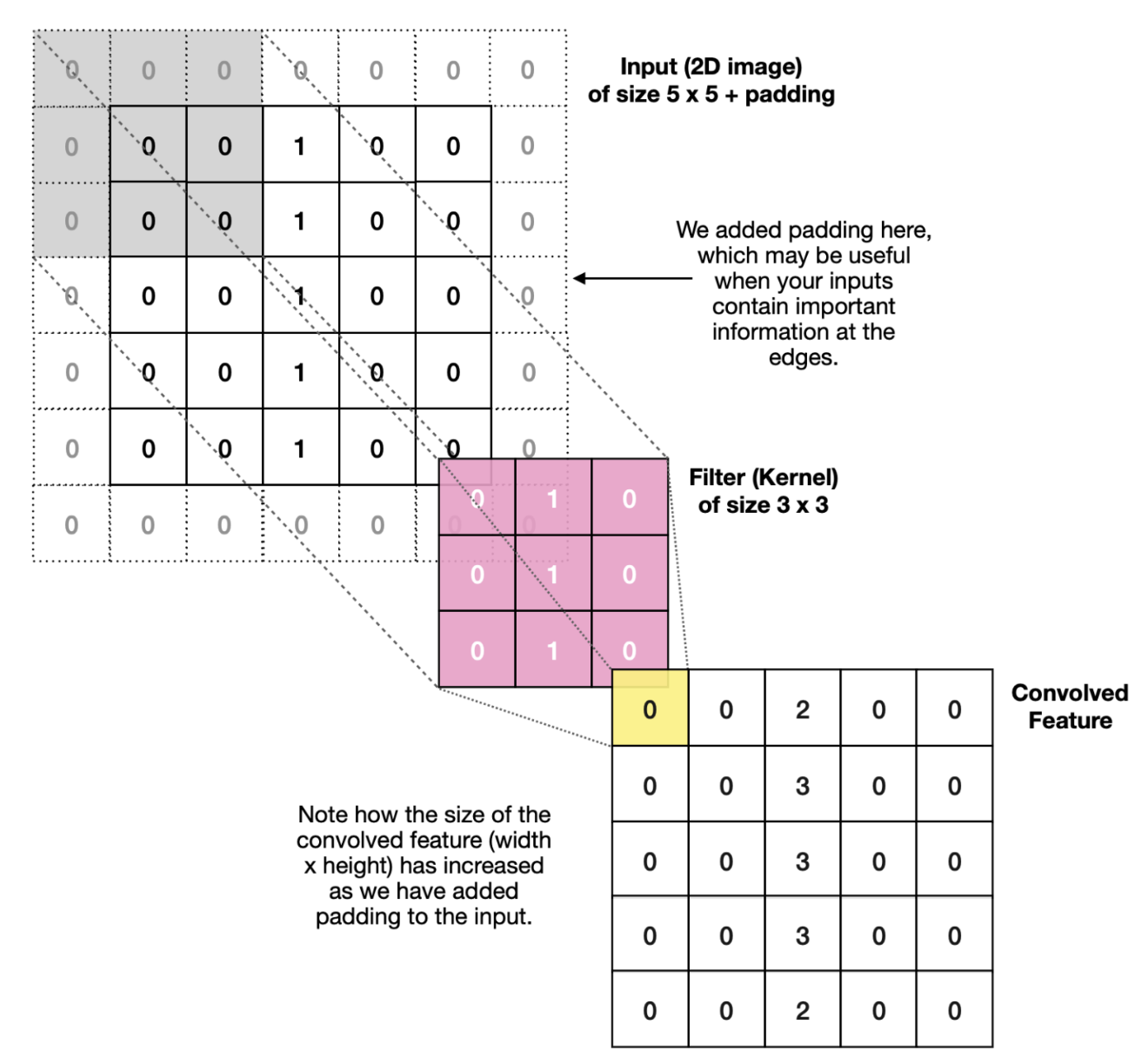
Weight sharing in CNNs

What does this mean for learning?
$\Rightarrow$ We have to learn the same thing in different locations!
$\Rightarrow$ An “edge” remains an “edge”, no matter where we are.
Instead of training a fully connected layer, we train the weights of a kernel that moves over the input
Same weights in every location $\Rightarrow$ weight sharing!

Architecture is closely related to fully connected NNs:
- Inner product between kernel weights $\theta$ and input $x$ $\Rightarrow$ activation $z$.
- Multiple kernels $\Rightarrow$ multiple channels.
- Then comes a nonlinear activation function $\sigma(z)$.
- Further followed by additional steps (see next slide).

images/06-deep-learning/CNN-kernels.gif — A kernel sweeping over an input [Source]

images/06-deep-learning/CNN-kernels_vertical.png — Second kernel = second channel [Source]

Ingredients of a CNN

Further considerations (padding & stride) and additional steps (e.g., pooling)

images/06-deep-learning/CNN-padding.png — Padding [Source]

images/06-deep-learning/CNN-stride.gif — Stride [Source]

images/06-deep-learning/CNN-pooling.gif Pooling [Source]

Neural network architectures

images/06-deep-learning/NN-zoo2.png — The neural network zoo [Asimov Institute].

Linear regression as a special case

The linear model: single-layer NN with $\sigma=\mathsf{Id}$

Let’s assume that we only have a single layer directly mapping inputs $x\in\R^n$ to outputs $y\in\R^m$: \[ \hat{y} = f_\Theta(x) = \Theta^\top x\qquad\text{with}\quad \Theta\in\R^{m\times n}.\]
Let’s consider the usual MSE loss: \[ L(\Theta) = \frac{1}{N} \sum_{k=1}^N \norm{\Theta^\top x_k - y_k}_2^2.\]
We organize the data in a slightly different fashion, i.e., \[ X = \begin{pmatrix} - & x_1^\top & - \\ & \vdots & \\ - & x_N^\top & - \end{pmatrix}\in\R^{N\times n}, \qquad Y = \begin{pmatrix} - & y_1^\top & - \\ & \vdots & \\ - & y_N^\top & - \end{pmatrix}\in\R^{N\times m}.\]
Then the model can predict all $N$ samples at the same time by a matrix-matrix product: $\hat{Y} = X\Theta$.
The associated loss function then simply is the Frobenius norm over the dataset $\Dtrain = (X,Y)$: \[ L(\Theta; \Dtrain) = \frac{1}{N} \norm{X\Theta - Y}_F^2 = \frac{1}{N} (X\Theta - Y)^\top (X\Theta - Y). \]

Solving the regression problem

What’s the necessary condition for the minimizer of a function?
$\Rightarrow$ The gradient has to be zero! \[ \pdiff{L(\Theta; \Dtrain)}{\Theta} = \pdiff{}{\Theta} \left[\frac{1}{N} (X\Theta - Y)^\top (X\Theta - Y) \right] = \frac{2}{N} X^\top (X\Theta - Y) \]
Optimal solution: \[\begin{align*} \frac{2}{N} X^\top (X\Theta^* - Y) &\stackrel{!}{=} 0 \\ \Leftrightarrow \quad X^\top X \Theta^* &= X^\top Y \\ \Leftrightarrow \quad \Theta^* &= (X^\top X)^{-1} X^\top Y = X^\dagger Y, \end{align*}\] where $X^\dagger$ is the pseudo-inverse of $X$.
Training is replaced by a simple one-step learning approach (using, e.g. numpy.linalg.pinv).
Since the loss function $L$ is convex, the solution $\Theta^*$ is not a local, but the global optimum.

Features as an additional pre-processing step

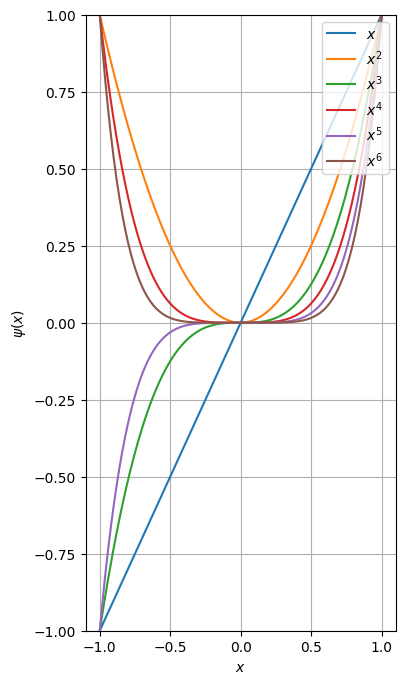
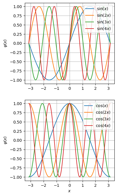
If we introduce feature functions $\psi_i:\R^n \rightarrow \R$, $\psi_i(x) = z_i$, then we can significantly improve the performance: \[ \psi(x) = [\psi_1(x), \ldots, \psi_q(x)]^\top. \]
Different ways of introducing features:

images/06-deep-learning/feature-engineering-linear.svg — Tailored (Abdelwanis et al. 2026)

images/06-deep-learning/Poly-features.png — Manual: Polynomials

images/06-deep-learning/Fourier-features.png — Manual: Fourier modes

images/06-deep-learning/ELM.svg — Randomly: Extreme Leraning Machine

Summary / what you have learned

There are three main learning paradigms:
- supervised learning for function approximation of input-to-output mappings,
- unsupervised learning for clustering, pattern detection or dimensionality reduction,
- reinforcement learning for sequential decision making in dynamic envionments.
In supervised learning, we aim to approximate an unknown function $f$ by a parametric function $f_\theta$ by adjusting $\theta$ such that a loss function $L$ is minimized over a training dataset $\Dtrain$.
- The central goal is generalization beyond the training data.
- We have to handle the bias-variance-tradeoff, which is often a matter of model complexity.
- There are many techniques to improve learning such as cross-validation, regularization, inductive biases, …
Deep neural networks come in a great range of varieties.
- They are a large network of a single unit known as the perceptron.
- The general structure consists of linear transformations, followed by nonlinear activation functions.
- Training is realized via backpropagation and gradient descent.
- Various versions for the descent direction, for instance using momentum.
- Improved efficiency (at the cost of noise) by using stochastic gradient descent or mini-batch gradient descent.
Linear regression is the special case of a single linear layer.
- Training can be realized in closed form using the pseudo-inverse.
- Features significantly improve the performance of linear models.

References

Abdelwanis, Ali, Barnabas Haucke-Korber, Darius Jakobeit, Wilhelm Kirchgässner, Marvin Meyer, Maximilian Schenke, Hendrik Vater, Oliver Wallscheid, and Daniel Weber. 2026. “Reinforcement Learning: A Comprehensive Open-Source Course.” Journal of Open Source Education 9 (97). The Open Journal: 306. doi:10.21105/jose.00306.

Abu-Mostafa, Yaser S, Malik Magdon-Ismail, and Hsuan-Tien Lin. 2012. Learning from Data. Vol. 4. AMLBook New York.

Bengio, Yoshua, Ian Goodfellow, Aaron Courville, et al. 2017. Deep Learning. Vol. 1. MIT press Cambridge, MA, USA.

Bishop, Christopher M. 2006. Pattern Recognition and Machine Learning. Vol. 4. 4. Springer.

Bronstein, Michael M., Joan Bruna, Taco Cohen, and Petar Veličković. 2021. “Geometric Deep Learning: Grids, Groups, Graphs, Geodesics, and Gauges.” arXiv:2104.13478, April.

Hastie, Trevor. 2009. “The Elements of Statistical Learning: Data Mining, Inference, and Prediction.” springer.

Kingma, Diederik P, and Jimmy Ba. 2014. “Adam: A Method for Stochastic Optimization.” arXiv Preprint arXiv:1412.6980.

Li, Hao, Zheng Xu, Gavin Taylor, Christoph Studer, and Tom Goldstein. 2018. “Visualizing the Loss Landscape of Neural Nets.” Advances in Neural Information Processing Systems 31.

Deep Reinforcement Learning

Brief Introduction to Deep Learning

Content

Content

Where are we?

The three main learning paradigms

The three main learning paradigms

Supervised learning

The learning diagram

Generalization

Supervised learning

Bias-variance tradeoff (1)

Bias-variance tradeoff (2)

Cross-validation

Means to improve a supervised learning model

Deep neural networks

Artificial neural networks

Multi-layer perceptron

Activation functions

Training (1)

Training (2)

Backpropagation example

Stochastic gradient descent and batch learning

Regularization

Convolutional neural networks

Ingredients of a CNN

Neural network architectures

Linear regression as a special case

The linear model: single-layer NN with \(\sigma=\mathsf{Id}\)

Solving the regression problem

Features as an additional pre-processing step

Summary / what you have learned

Summary / what you have learned

References