Deep Reinforcement Learning

Deep Q Learning

Prof. Dr. Sebastian Peitz

Chair of Safe Autonomous Systems, TU Dortmund

Summer term 2026

🚀 by Decker

Content

Recap:
- Tabular SARSA & $Q$-learning
- Value function approximation with NNs
On-policy control with gradients and semi-gradients
Deep Q networks (DQN)
- Extensions & modifications
Least squares policy iteration

Where are we?

Lecture contents
Chapter	Topic	Content
	Basics & tabular methods
1-5	Bandits, MDPs, Dynamic Programming, Monte Carlo, TD Learning	RL basics in finite dimensions
	Deep-learning-based methods
6	Brief introduction to deep learning	The basics for what comes next
7	Value function approximation	Value estimation with function approximation
8	Deep $Q$-learning	$Q$-learning with neural networks
9	Policy gradients
10	Actor-critic algorithms
11	Advanced algorithms (Part I): From policy gradient to PPO
12	Advanced algorithms (Part II): From $Q$-learning to Soft Actor-Critic
	Model-Based Control
	Advanced Topics

Recap: Tabular SARSA and $Q$-learning

Tabular SARSA and $Q$-learning

Algorithm: SARSA (On-policy).

initialize

$Q(s,a)$ arbitrarily for $s \in \Sc, a \in \Ac$
$Q(\terminal,\cdot) = 0$
$\pi = \epsilon$-greedy$(Q)$

for $k = 1, 2, \ldots, K$ episodes:
$\quad$ Initialize $s_t \gets s_0$, $t \gets 0$
$\quad$ while $s_t$ is not terminal:
$\quad\quad$ Take action $a_t \sim \pi(s_t)$ and observe $(r_t,s_{t+1})$
$\quad\quad$ Select $a_{t+1} \sim \pi(s_{t+1})$
$\quad\quad$ Update $Q$ given $(s_t,a_t,r_t,s_{t+1},a_{t+1})$: $\quad$ \[Q(s_t,a_t) \gets Q(s_t,a_t) + \alpha \left[r_t + \gamma \textcolor{blue}{Q(s_{t+1},a_{t+1})}- Q(s_t,a_t)\right]\] $\quad\quad$ Update policy: $\pi = \epsilon$-greedy$(Q)$
$\quad\quad$ $t \gets t+1$

Algorithm: $Q$-learning (Off-policy).

initialize

$Q(s,a)$ arbitrarily for $s \in \Sc, a \in \Ac$
$Q(\terminal,\cdot) = 0$
$\pi = \epsilon$-greedy$(Q)$

for $k = 1, 2, \ldots, K$ episodes:
$\quad$ Initialize $s_t \gets s_0$, $t \gets 0$
$\quad$ while $s_t$ is not terminal:
$\quad\quad$ Take action $a_t \sim \pi(s_t)$ and observe $(r_t,s_{t+1})$
$\quad\quad$ ~~Select $\cancel{a_{t+1} \sim \pi(s_{t+1})}$~~
$\quad\quad$ Update $Q$ given $(s_t,a_t,r_t,s_{t+1})$: $\quad$ \[Q(s_t,a_t) \gets Q(s_t,a_t) + \alpha \left[r_t + \gamma \textcolor{red}{\max_a Q(s_{t+1},a)}- Q(s_t,a_t)\right]\] $\quad\quad$ Update policy $\pi = \epsilon$-greedy$(Q)$
$\quad\quad$ $t \gets t+1$

Tabular SARSA and $Q$-learning: Gridworld

On-policy: SARSA

Off-policy: $Q$-learning

Discount: $\gamma = 0.9$
Exploration: $\epsilon = 0.2$
Step size: $\alpha = 0.5$

Recap: Value function approximation

We want to approximate the value function by parametric model with trainable parameters $\theta\in\R^d$, i.e., $V_\theta(s) \approx V^\pi(s)$.
For training, we need to define a prediction objective: \[\begin{equation} L(\theta) = \sum_{k=1}^N \big(V^\pi(s_k) - V_\theta(s_k)\big)^2 \approx \int_\Sc \mu(s) \big(V^\pi(s) - V_\theta(s)\big)^2 \ds = \overline{VE}(\theta). \label{eq:DQL_V_L} \end{equation}\]
Incremental weight updates via
- gradients, e.g., in the Monte Carlo setting: \[\begin{equation} \theta \gets \theta + \alpha\rbracket{g - V_\theta(s)} \nablatheta V_\theta(s). \label{eq:DQL_V_update_MC} \end{equation}\]
- semi-gradients in the bootstrapping case: we are not differentiating the target, which also depends on $V_\theta$. For TD learning, we have \[\begin{equation} \theta \gets \theta + \alpha\rbracket{r + \gamma V_\theta(s') - V_\theta(s)} \nablatheta V_\theta(s). \label{eq:DQL_V_update_TD} \end{equation}\]
Batch updates using $\Bc=\set{(s_i, r_i,s'_i)}_{i=1}^b \subset\Dc$ instead of a single sample as in SGD. For TD updates, we thus get \[ \begin{equation} \theta \gets \theta + \frac{\alpha}{b} \sum_{(s_i, r_i,s'_i)\in\Bc} \rbracket{r_i + \gamma V_\theta(s'_i) - V_{\theta}(s_i)} \nablatheta V_{\theta}(s_i). \label{eq:DQL_V_update_TD_batch} \end{equation}\]
For linear models (i.e., $V_{\theta}(s) = \theta^\top \psi(s) = \sum_{k=1}^d \theta_k \psi_k(s)$), training can be done in one step via linear regression: \[ \begin{equation} \theta^* = (\Psi^\top \Psi)^{-1} \Psi^\top y = \Psi^\dagger y \qquad \Rightarrow \qquad V_{\theta^*}(s) = {\theta^*}^\top \psi(s) = \sum_{k=1}^d \theta^*_k \psi_k(s) . \label{eq:DQL_V_LSQ} \end{equation}\]

On-policy control with gradients and semi-gradients

Value-based control: $Q$-function approximation

Today’s focus: value-based control $\Rightarrow$ How to transfer tabular methods to the function approximation case.

The states are continuous, but the actions are (usually) still discrete.
Central object of interest: The Q function that we wish to approximate with a parametric model (e.g., a neural net) \[ Q_\theta (s,a) \approx Q^\pi(s,a) \]
We can then use this in the well-known generalized policy iteration (GPI) scheme to identify optimal policies: \[ Q_\theta(s,a) \approx Q^*(s,a) \quad \Rightarrow \quad \pi^*(s) = \arg\max_{a\in\Ac} Q_\theta(s,a) .\]

Types of architectures (Abdelwanis et al. 2026)

Gradient-based action value learning

The transfer from value function approximation is straightforward!

Adaptation of $\eqref{eq:DQL_V_L}$ to get $L(\theta)$ \[\begin{equation} L(\theta) = \sum_{k=1}^N \big(Q^\pi(s_k, a_k) - Q_\theta(s_k, a_k)\big)^2 . \label{eq:DQL_Q_L} \end{equation}\]
Incremental update using (semi-)gradients: \[ \begin{equation} \theta \gets \theta + \alpha\rbracket{Q^\pi(s,a) - Q_\theta(s,a)} \nablatheta Q_\theta(s,a). \label{eq:DQL_Q_update} \end{equation} \]
Depending on the control approach, the true target $Q^\pi(s, a)$ is approximated by:
- Monte Carlo: full episodic return \[Q^\pi(s,a) \approx g,\]
- SARSA: one-step bootstrapped estimate \[Q^\pi(s,a) \approx r + \gamma Q_\theta(s',a'),\]
- $n$-step SARSA: \[Q^\pi(s_t, a_t) \approx r_t + \gamma r_{t+1} + \ldots + \gamma^{n-1} r_{t+n-1} + \gamma^n Q_\theta(s_{t+n},a_{t+n}).\]

Algorithm: Gradient MC control

Algorithm: Gradient Monte Carlo algorithm for estimating $Q^\pi$ / $Q^*$

Input:

a differentiable, parameter-dependent function $Q_\theta: \Sc \times \Ac \to \R$
learning rate $\alpha$
Prediction case: a policy $\pi$
Improvement case: $\epsilon$ defining the $\epsilon$-greedy policy update based on $Q_\theta$

Initialize: Value function weights $\theta\in\R^d$ arbitrarily

for $k = 1, 2, \ldots, K$ episodes:
$\quad$ Generate a sequence following $\pi$ (or $\epsilon$-greedy$(Q_\theta)$): \[((s_0,a_0,r_0),(s_1,a_1,r_1),\ldots,(s_{T_k-1},a_{T_k-1},r_{T_k-1}))\] $\quad$ Calculate the every-visit returns $g_t$
$\quad$ for $t = 0,1,\ldots,T-1$:
$\quad\quad$ $\theta \gets \theta + \alpha\rbracket{g_t - Q_\theta(s_t,a_t)} \nablatheta Q_\theta(s_t,a_t)$

Direct transfer from tabular case to function approximation.
Update target becomes the sampled return $Q^\pi(s_t, a_t) \approx g_t$.
If operating $\epsilon$-greedy on $Q_\theta$: baseline policy (given by $\iterate{\theta}{0}$) must terminate the episode!

Algorithm: Semi-gradient SARSA

Algorithm: Semi-gradient SARSA for estimating $\textcolor{red}{Q^\pi}$ / $\textcolor{blue}{Q^*}$

Input:

a differentiable, parameter-dependent function $Q_\theta: \Sc \times \Ac \to \R$
learning rate $\alpha$
Prediction case: a policy $\pi$
Improvement case: $\epsilon$ defining the $\epsilon$-greedy policy update based on $Q_\theta$

Initialize: Value function weights $\theta\in\R^d$ arbitrarily

for $k = 1, 2, \ldots, K$ episodes:
$\quad$ Initialize $s_0$
$\quad$ for $t = 0,1,\ldots,T-1$:
$\quad\quad$ Obtain $\textcolor{red}{a_t \sim \policy{\cdot}{s_t}}$ (or $a_t \sim \epsilon$-greedy$(Q_\theta(s_t,\cdot))$)
$\quad\quad$ Observe $r_t$ and $s_{t+1}$
$\quad\quad$ if $s_{t+1}$ is $\terminal$ then
$\quad\quad\quad$ $\theta \gets \theta + \alpha\rbracket{r_t - Q_\theta(s_t,a_t)} \nablatheta Q_\theta(s_t,a_t)$
$\quad\quad\quad$ Go to next episode $k+1$
$\quad\quad$ Choose $a_{t+1} \sim \policy{\cdot}{s_{t+1}}$ (or $a_{t+1} \sim \epsilon$-greedy$(Q_\theta(s_{t+1},\cdot))$)
$\quad\quad$ $\theta \gets \theta + \alpha\rbracket{r_t + \gamma Q_\theta(s_{t+1},a_{t+1}) - Q_\theta(s_t,a_t)} \nablatheta Q_\theta(s_t,a_t)$

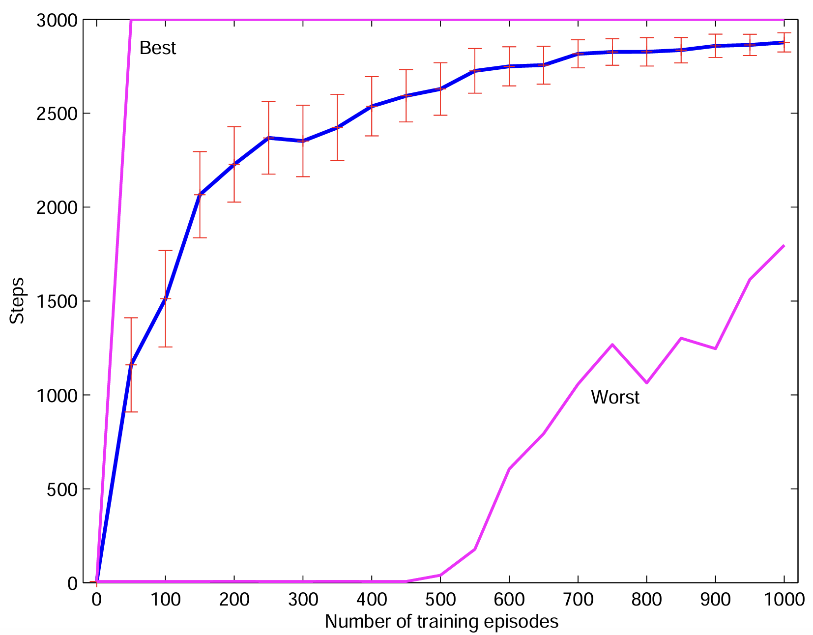
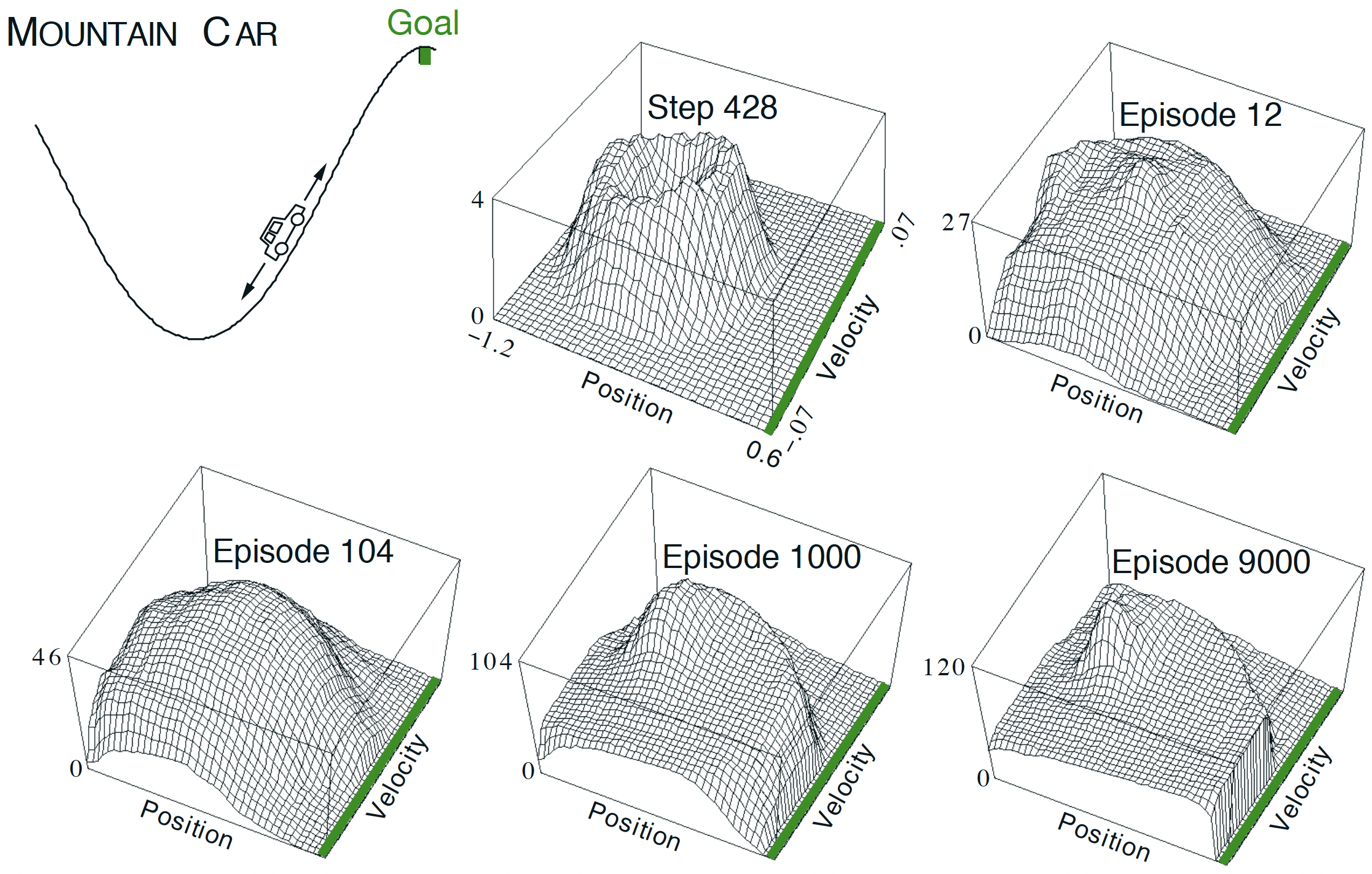
Example: Mountain car (1)

Continous state $s\in\Sc=[\submin{x},\submax{x}]\times[\submin{v},\submax{v}]$ (minimal and maximal position $x$ and velocity $v$).
Single, discrete action $a\in\Ac=\set{-1,0,1}$.
$r = −1$ (goal is to terminate episode as quick as possible).
Episode terminates when car reaches the flag (or max steps).
Simplified longitudinal car physics with state constraints.
Position initialized randomly within valley, zero initial velocity.
Car is underpowered and requires swing-up.

images/07-value-approximation/Mountain-car.gif — Mountain car (Sutton and Barto 1998, Gymnasium)

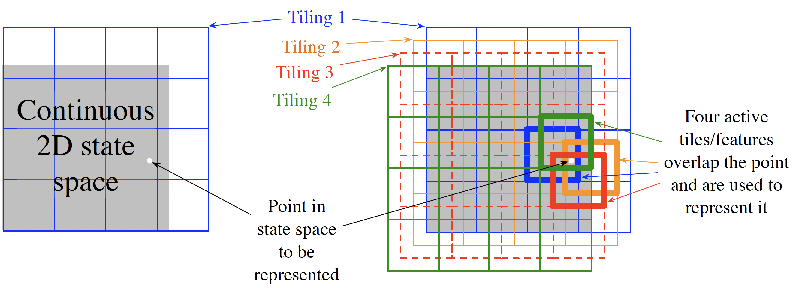
Approximation: Linear model with tile coding features $x_i(s,a)$, where \[ \begin{align*} \psi(s,a)&=\sum_{i=1}^d \theta_i x_i(s,a), \\ x_i(s,a)&=\begin{cases} 1 & (s,a)\in\text{ tile \#}i \\ 0 & \text{otherwise} \end{cases}. \end{align*} \]

images/08-deep-q-learning/tile_coding.png — Tile coding (Sutton and Barto 1998, Figure 9.9)

Example: Mountain car (2)

images/08-deep-q-learning/mountain_car_results.png — The Mountain Car task (upper left panel) and the cost-to-go function ($−\max_{a\in\Ac} Q_\theta(s, a,)$) learned during one run. (Sutton and Barto 1998, Figur 10.1)

Warning: a huge drawback of function approximation

Recall tabular policy improvement theorem: guarantee to find a globally better or equally good policy in each update step.
Parameter updates of the form $\eqref{eq:DQL_Q_update}$ have an impact on $Q(s,a)$ for all $s$ and $a$, not just the one we visited!

images/08-deep-q-learning/SuttonBarto_GPI.svg — Generalized Policy Iteration (GPI) (Sutton and Barto 1998)

Loss of the policy improvement theorem

When using function approximation, the policy improvement theorem does no longer apply.
While improving the policy, we may impair it in other places at the same time.

Deep $Q$ networks (DQN)

General strategy behind DQN

Introduced in the famous DeepMind paper (Mnih et al. 2015).
Same off-policy strategy as in the classical/tabular $Q$-learning algorithm: \[Q(s,a) \gets Q(s,a) + \alpha \left[r + \gamma \max_{a'\in\Ac} Q(s',a')- Q(s,a)\right].\]
Now: incremental learning using semi-gradients (Eq. $\eqref{eq:DQL_Q_update}$) and TD($0$) bootstrapping: \[ \begin{equation} \theta \gets \theta + \alpha\rbracket{r + \gamma \max_{a'\in\Ac} Q_\theta(s',a') - Q_\theta(s,a)} \nablatheta Q_\theta(s,a). \label{eq:DQL_DQN-gradient} \end{equation} \]

But with two important distinctions

An experience replay buffer for batch learning replaces the single-sample updates.
A separate set of weights $\theta'$ for the bootstrapped Q-target ($\eqref{eq:DQL_DQN-gradient}$ is not a gradient).

The motivation behind this

Sample efficiency

Experience replay: efficiently use available data.
Stabilize learning by reducing the correlation between samples
$\Rightarrow$ sampling from a replay buffer leads to i.i.d.-like data.

Stabilization of learning

targets don’t change in inner loop $\Rightarrow$ well-defined learning problem.

DQN working principle (1)

Take actions u based on $Q_\theta(s,a)$ (e.g., $\epsilon$-greedy).
Store observed tuples $(s,a,r,s')$ in memory buffer $\Dc$.
Sample mini-batches $\Bc$ from $\Dc$.
Calculate bootstrapped Q-target with a target network with weights $\theta'$: \[ Q^\pi(s,a)\approx r + \max_{a\in\Ac}Q_{\theta'}(s,a). \]
Optimize MSE loss between above targets and the regular approximation $Q_{\theta}(s,a)$ using $(s_i,a_i,r_i,s_i')\in\Bc$: \[ \begin{align*} L(\theta) &= \sum_{i=1}^{\abs{\Bc}} \big(\underbrace{r_i + \max_{a\in\Ac}Q_{\theta'}(s_i',a)}_{=y_i~(\target)} - Q_{\theta}(s_i,a_i)\big)^2, \\ \theta &\gets \theta + \alpha \sum_{i=1}^{\abs{\Bc}} \rbracket{y_i - Q_\theta(s_i,a_i)} \nablatheta Q_\theta(s_i,a_i). \end{align*} \]
Update $\theta'$ based on $\theta$ from time to time.

DQN working principle (2)

Adapted from (Abdelwanis et al. 2026)

The DQN algorithm

Algorithm: The “classic” DQN algorithm (Mnih et al. 2015)

Input:

a differentiable, parameter-dependent function $Q_\theta: \Sc \times \Ac \to \R$
learning rate $\alpha$, greedy parameter $\epsilon$, update rate $N_\theta\in\N$

Initialize: Q function weights $\theta = \theta' \in\R^d$ arbitrarily, $\Dc=\{\}$

for $k = 1, 2, \ldots, K$ episodes:
$\quad$ Initialize $s_0$
$\quad$ for $t = 0,1,\ldots,T-1$:
$\quad\quad$ Obtain $a_t \sim \epsilon$-greedy$(Q_\theta(s_t,\cdot))$ and observe $r_t$ and $s_{t+1}$
$\quad\quad$ Store tuple $(s_t,a_t,r_t,s_{t+1})$ in $\Dc$
$\quad\quad$ Sample minibatch $\Bc$ from $\Dc$ (after initial warm-up)$\qquad\qquad\qquad$
$\quad\quad$ Compute targets for $(s_i,a_i,r_i,s'_i)\in\Bc$ \[y_i = r_i + \max_{a\in\Ac}Q_{\theta'}(s_i',a) \qquad\text{(or}~y_i = r_i~\text{if $s'_{i}$ is terminal)}\] $\quad\quad$ Update $\theta$ via gradient descent on $L(\theta)$ with learning rate $\alpha$
$\quad\quad$ if $t\mod{N_\theta}=0$ then $\theta'\gets\theta$

Remarks:

For the standard MSE loss \[L(\theta)= \sum_{i=1}^{\abs{\Bc}} \big(y_i - Q_{\theta}(s_i,a_i)\big)^2,\] the weight update becomes the one we have seen before: \[\theta \gets \theta + \alpha \sum_{i=1}^{\abs{\Bc}} \rbracket{y_i - Q_\theta(s_i,a_i)} \nablatheta Q_\theta(s_i,a_i).\]
Apart from standard gradient descent, advanced (i.e., momentum-based) descent algorithms are possible (e.g., RMSProp, Adam, …)

Example: Atari game Pong (1)

State $s$:
- $210 \times 160$ pixels with $3$ channels each (RGB) and values $s_{i}\in\{0,\ldots,255\}$,
- stacking of multiple frames,
- some additional preprocessing.
Action $a$: $18$ actions in total, ($6$ buttons, some of which can be pushed at the same time).
Architecture for $Q_\theta$ (Mnih et al. 2015):
$\qquad$
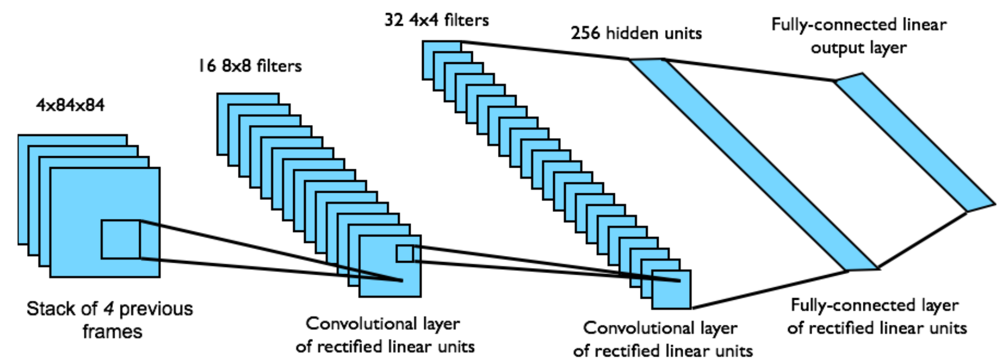
Loss function $L(\theta)$: Huber loss $L_\beta(\theta) = \begin{cases} \frac{1}{2}\theta^2, & \theta \leq \beta \\ \beta(\abs{\theta} - \frac{1}{2}\theta), & \text{otherwise} \end{cases}$.
Training: RMSProp descent algorithm.
Annealing of the exploration rate: $\epsilon$ goes from $1$ to $0.1$ (or $0.05$) over the first $10^6$ frames.

videos/08-deep-q-learning/DQN_Pong/pong.gif — Pong setup: More details in the Farama Gymnasium description.

images/08-deep-q-learning/Huber_loss.svg — Huber loss (Wikipedia)

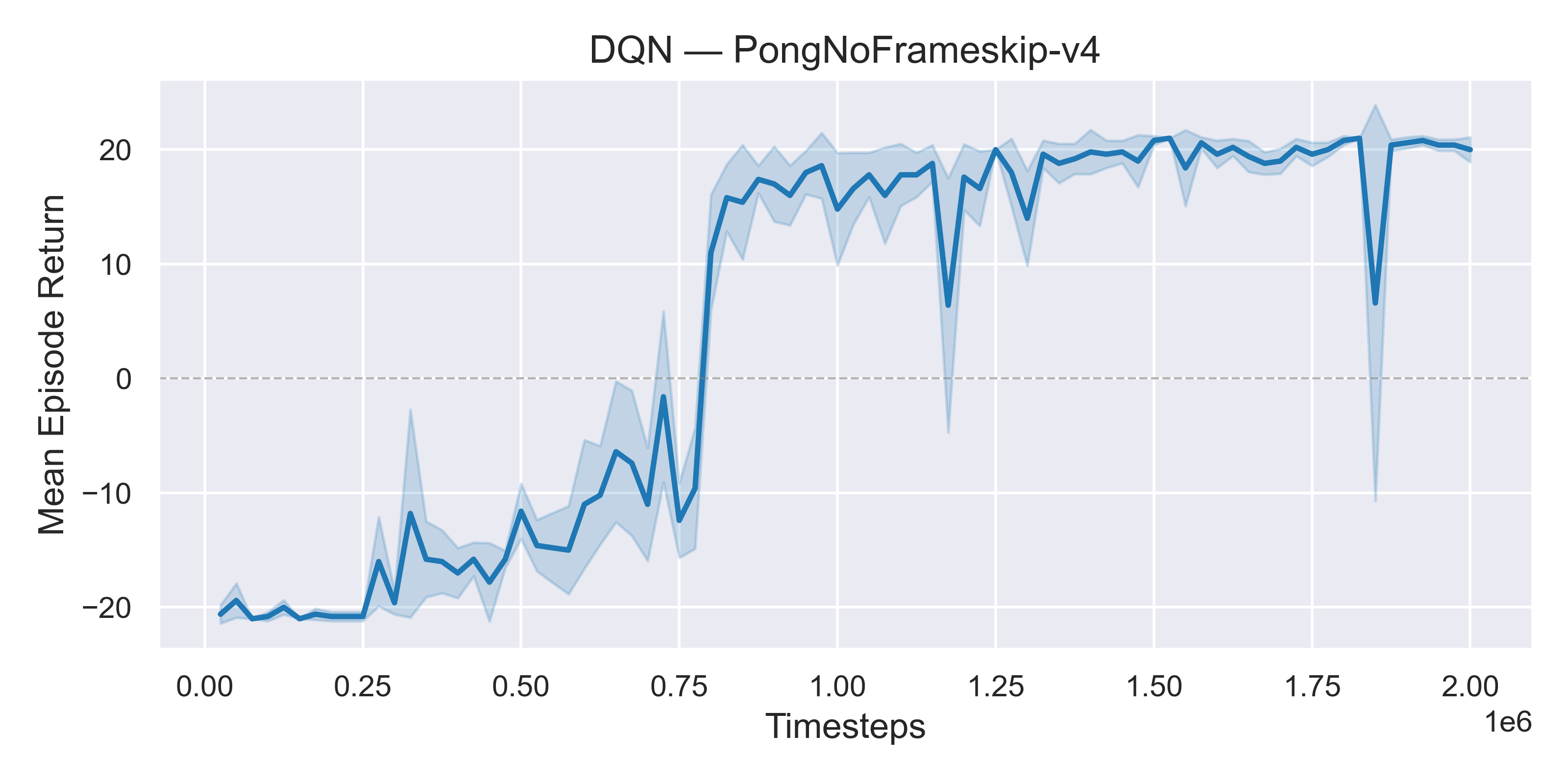
Example: Atari game Pong (2)

videos/08-deep-q-learning/DQN_Pong/rl_model_0_steps.gif — 0 steps

videos/08-deep-q-learning/DQN_Pong/rl_model_100000_steps.gif 100,000 steps

videos/08-deep-q-learning/DQN_Pong/rl_model_300000_steps.gif 300,000 steps

videos/08-deep-q-learning/DQN_Pong/rl_model_500000_steps.gif 500,000 steps

videos/08-deep-q-learning/DQN_Pong/rl_model_800000_steps.gif 800,000 steps

videos/08-deep-q-learning/DQN_Pong/rl_model_1000000_steps.gif 1,000,000 steps

videos/08-deep-q-learning/DQN_Pong/rl_model_1500000_steps.gif 1,500,000 steps

videos/08-deep-q-learning/DQN_Pong/rl_model_2000000_steps.gif 2,000,000 steps

videos/08-deep-q-learning/DQN_Pong/dqn_PongNoFrameskip-v4_return.png — Return

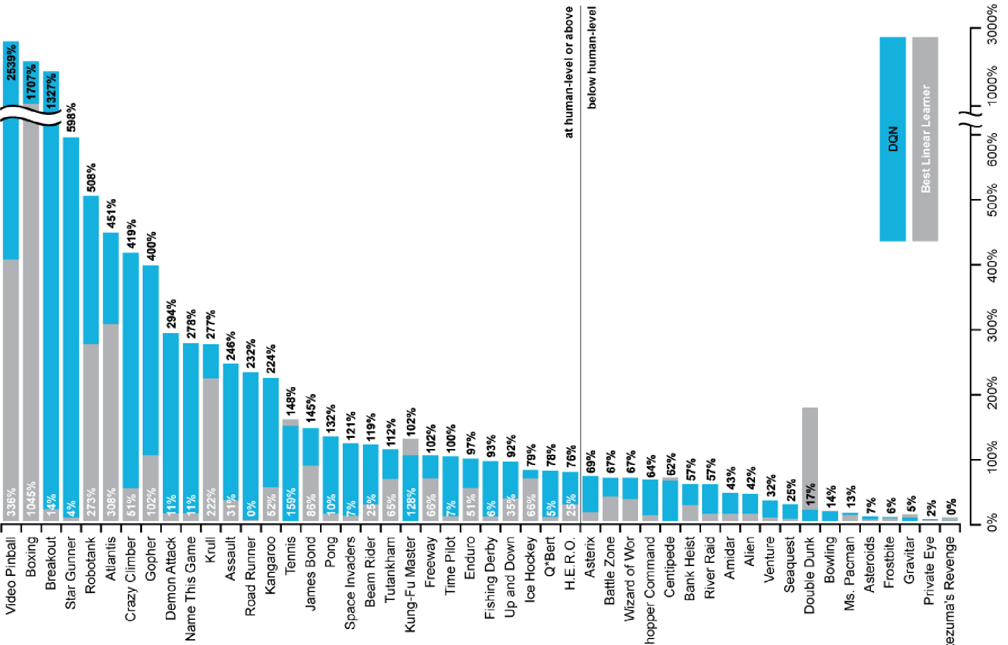
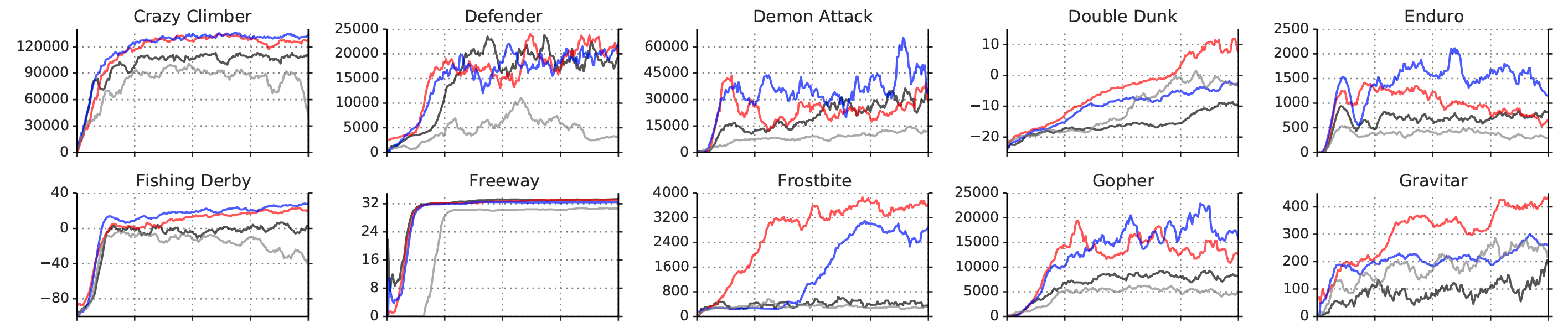
Example: Atari games

images/08-deep-q-learning/DQN_Atari_Results.png — Human-level control (Mnih et al. 2015)

The general view of $Q$-learning

Inspired by Sergey Levine’s CS285 lecture.

DQN: Processes 1 and 3 run at the same speed, process 2 is slower.
Online $Q$-learning: evict immediately, Process 1, 2 and 3 all run at the same speed.
- Value or $Q$-learning as in the last lecture, followed directly by a policy improvement step.
- Also similar to the value iteration algorithm from dynamic programming.
Many variations: data collection and eviction strategies, frequencies and repetitions of the individual process steps, …

DQN extensions & modifications

Alternative target networks (Polyak averaging)

Consider the DQN algorithm and separate it into three main components:
1. Data collection, i.e., store tuples $(s,a,r,s')$ in $\Dc$.
2. Improvement using mini batches $\Bc$ and a fixed target network, e.g., $\theta \gets \theta + \alpha \sum_{i=1}^{\abs{\Bc}} \rbracket{y_i - Q_\theta(s_i,a_i)} \nablatheta Q_\theta(s_i,a_i)$.
3. Update target network every $N_\theta$ steps: $\theta' \gets \theta$.
Let’s visualize these steps (with $N_\theta=4$, even though it’s usually much larger):
The lag is different in different places! This doesn’t need to be a problem, but it feels uneven.
Alternative: Polyak averaging. In every step, perform the linear interpolation \[ \theta' \gets \tau\theta' + (1-\tau) \theta \]
When initializing $\theta'=\theta$, this linear interpolation tends to work for nonlinear models (i.e., NNs) as well!

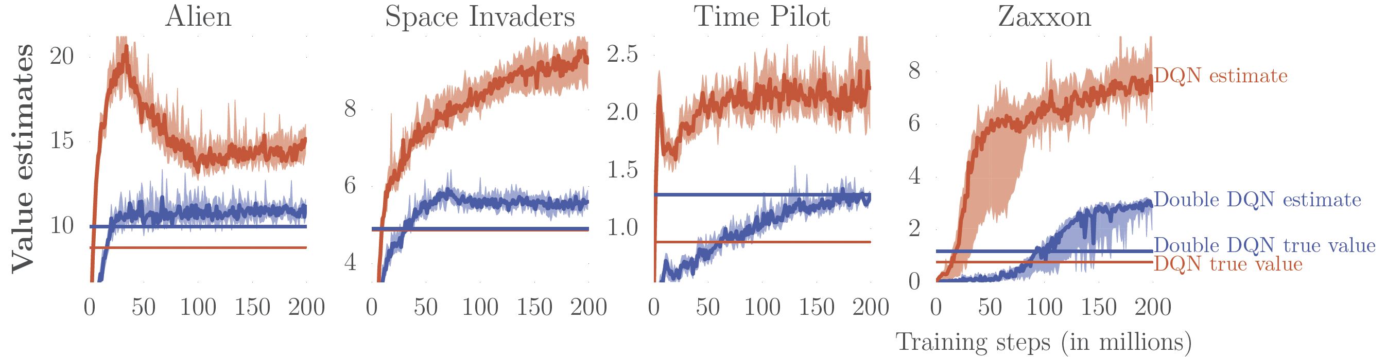
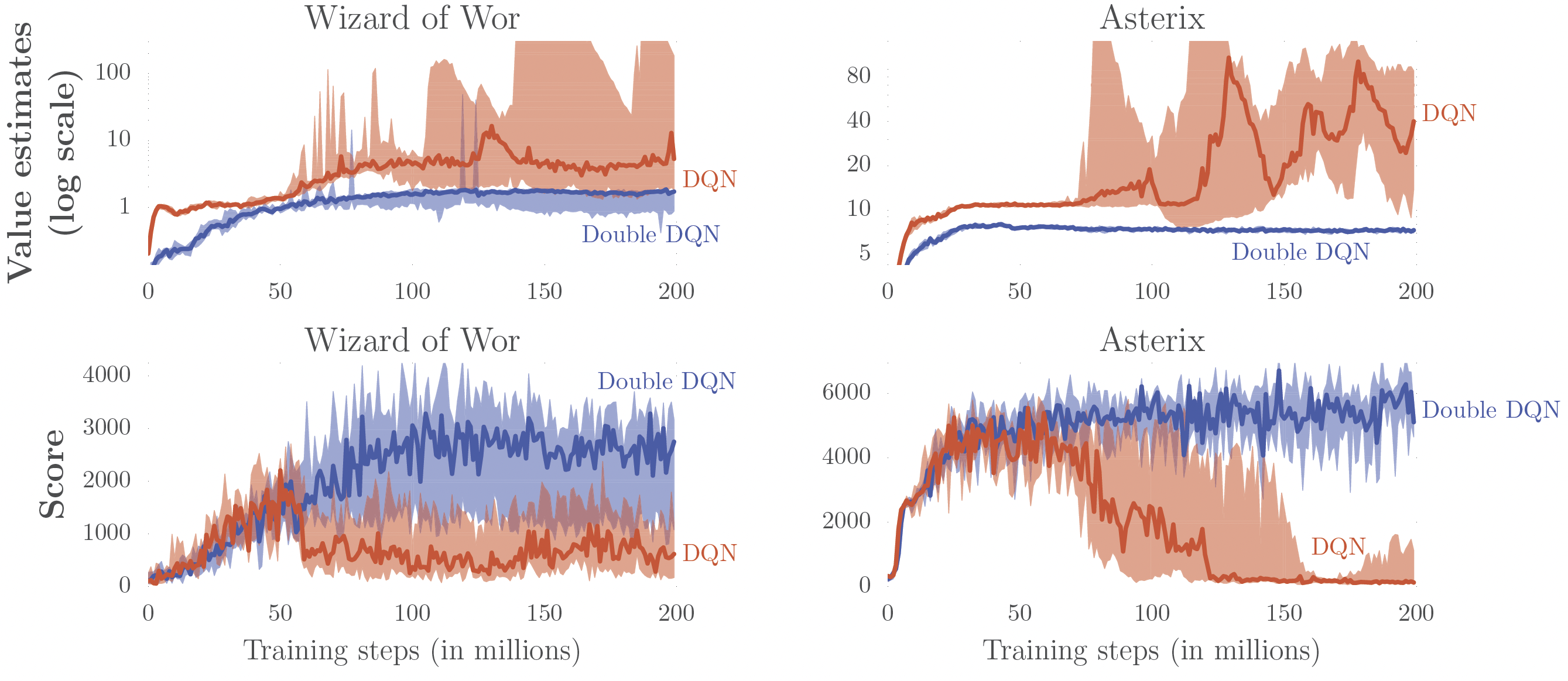
Double $Q$ networks (Hasselt, Guez, and Silver 2016)

Remember the maximization bias and double $Q$-learning?
$\Rightarrow$ Don’t use same network to choose the action and estimate the value!

Double deep $Q$-learning:

Just use the current network ($\theta$) to evaluate the action.
Still use the target network ($\theta'$) to evaluate the value. \[y = r + \gamma \textcolor{red}{Q_{\theta'}}(s',\arg\max_{a\in\Ac} \textcolor{blue}{Q_\theta}(s',a))\]

Algorithm recap: Tabular Q-Learning.

Take $a_t$ ($\epsilon$-greedy on $Q_1 + Q_2$), observe $(r_t,s_{t+1})$
if $\mathsf{rand()} > 0.5$ then \[\begin{align*} &y = r_t + \gamma \textcolor{red}{Q_2}(s_{t+1},\arg\max_{a\in\Ac} \textcolor{red}{Q_1}(s_{t+1},a))\\ &Q_1(s_t,a_t) \gets Q_1(s_t,a_t) + \alpha \left[y - Q_1(s_t,a_t)\right] \end{align*}\]
else: …

images/08-deep-q-learning/DDQN-results1.png

images/08-deep-q-learning/DDQN-results2.png

Prioritized experience replay (Schaul et al. 2016)

Samples in the replay buffer are not equally important.
From some examples, you can learn more than from others.
What would be a good criterion to assess the relevance of a particular sample? $\Rightarrow$ The TD error \[\delta_i = r_i + \max_{a\in\Ac}Q_{\theta'}(s_i',a) - Q_\theta(s_i,a_i)\]

images/08-deep-q-learning/Q-learning-general.svg — Inspired by Sergey Levine’s CS285 lecture.

Instead of sampling uniformly from the replay buffer, we assign an individual probability to each sample: \[ P(i) = \frac{p_i^\alpha}{\sum_{k=1}^{\abs{\Dc}}p_k^\alpha}, \qquad p_i = \abs{\delta_i} + \epsilon.\]
- Here, $\alpha\geq 0$ determines the degree of prioritization ($\alpha=0$ is the uniform case).
- The parameter $\epsilon>0$ ensures that all samples are drawn with non-zero probability.
A version that’s less sensitive to outliers: rank the transitions according to $\abs{\delta_i}$: \[p_i = \frac{1}{\mathsf{rank}(i)}.\]
But: this introduces a bias (we sample from a different, uncontrollable distribution) $\Rightarrow$ Use importance sampling!

$n$-step returns

The concept of TD($n$) can be extended to deep $Q$-learning in a straightforward fashion: \[ y_t = r_t + \gamma r_{t+1} + \gamma^2 r_{t+2} + \ldots + \gamma^{n-1} r_{t+n-1} + \gamma^{n} \max_{a\in\Ac} Q_{\theta}(s_{t+n},a). \]

$\textcolor{green}{\mathbf{+}\text{ less biased target values when estimates using }Q_\theta\text{ are inaccurate}}$

$\textcolor{green}{\mathbf{+}\text{ typically faster learning, especially early on}}$

$\textcolor{red}{\mathbf{-}\text{ only actually correct when learning on policy}}$

Some remarks on continuous actions

What’s the problem with continuous actions in DQN?

The action selection: $\pias = \begin{cases} 1, & a = \arg\textcolor{red}{\max}_{a'\in\Ac} Q_\theta(s,a') \\ 0, & \text{otherwise} \end{cases}$ (or some $\epsilon$-greedy alternative).
The target calculation: $y_i = r_i + \textcolor{red}{\max}_{a\in\Ac}Q_{\theta'}(s_i',a)$.

$\Rightarrow$ if $\Ac$ is continuous (i.e., $a\in\R^m$), then the maximization becomes a challenging optimization probelm in itself!

What can we do?

Gradient based optimization (e.g., SGD) $\quad\Rightarrow\quad\textcolor{red}{\mathbf{-}\text{ This can be too slow!}}$
Simple sampling: \[\max_{a\in\Ac} Q(s,a) \approx \max\set{Q(s,a_1),\ldots,Q(s,a_p)}, \qquad \text{with}~\set{a_1,\ldots,a_p}\sim U(\Ac).\] $\Rightarrow$ $\quad\textcolor{green}{\mathbf{+}\text{ Very efficient.}}\quad$ $\textcolor{green}{\mathbf{+}\text{ Easily parallelized.}}\quad$ $\textcolor{red}{\mathbf{-}\text{ Not very accurate.}}$
Other stochastic optimization techniqes $~\quad\Rightarrow\quad\textcolor{red}{\mathbf{-}\text{ Usually also quite slow, or scale poorly.}}$
Train second network $\pi_\phi: \Sc \to \Ac$ whose output maximizes $Q_\theta(s,a)$: \[Q(s,\pi_\phi(s)) \approx \max_{a\in\Ac} Q_\theta(s,a)\fragment{ \qquad\Rightarrow\quad \text{Actor-critic methods (in two lectures)!}\qquad\qquad~~ }\]

Some practical tips

Following Sergey Levine’s CS285 lecture:

Q learning takes some care to stabilize.
- Test on easy, reliable tasks first, make sure your implementation is correct.
  (Schaul et al. 2016)
Large replay buffers help improve stability.
Looks more like fitted Q iteration.
It takes time, be patient; performance might be no better than random for a while.
Start with high exploration ($\epsilon$) and gradually reduce.

Bellman error gradients can be big; clip gradients or use Huber loss.
Double Q learning helps a lot in practice: it’s simple and has no downsides.
$n$-step returns also help a lot, but have some downsides.
Schedule exploration (high to low) and learning rates (high to low). The Adam optimizer can help too.
Run multiple random seeds, it’s very inconsistent between runs.

Least squares policy iteration

Linear action-value-function estimation

Recall the LSTD algorithm from last lecture: batch least squares estimation $V^\pi(s)$ with linear models: \[ y = \begin{bmatrix} r_0 \\ \vdots \\ r_{T-1} \end{bmatrix}, \quad \fragment{ \Psi = \begin{bmatrix} \psi_0^\top - \gamma \psi_1^\top\\ \vdots \\ \psi_{T-1}^\top - \gamma \psi_T^\top \end{bmatrix}, \quad } \fragment{ L(\theta) = \frac{1}{N} \norm{y - \Psi \theta }_F^2, \quad } \fragment{ \theta^* = (\Psi^\top \Psi)^{-1} \Psi^\top y = \Psi^\dagger y, \quad } \fragment{ V_{\theta^*}(s) = {\theta^*}^\top \psi(s). }\]
Let’s do the same for Q values $\Rightarrow$ LS-SARSA / LSTD$\mathbf Q$ \[ \begin{align*} Q_\theta(s,a) &= \theta^\top \psi(s,a) = \sum_{i=1}^d \theta_i \psi_i(s,a) \qquad &&\text{(Linear model)} \\ Q^\pi(s,a) &\approx r + \gamma Q_\theta(s', a') \qquad &&\text{(TD($0$) bootstrapping)} \end{align*}\]
Loss function: \[ L(\theta) = \sum_{t=0}^T \big(r_t - \rbracket{\psi^\top_{t} - \gamma \psi^\top_{t+1}} \theta\big)^2 = \frac{1}{N} \norm{y - \Psi \theta }_F^2, \qquad\text{where}~\psi_t = \psi(s_t,a_t) . \]
Same as before, only that the features depend on both states and actions: $\psi(s,a)$.

On-policy and off-policy LS-SARSA

Same data collection procedure as before: batch mode $\Rightarrow$ $\Psi$ and $y$.
Regarding the data in $\Psi$, we can distinguish two cases:
- the same policy $\pi$ (on-policy learning),
- an arbitrary policy $a'\sim \pi'\agivenb{\cdot}{s'}$ (off-policy learning).
If we apply off-policy LS-SARSA then
- we retrieve the flexibility to collect training samples arbitrarily,
- at the cost of an estimation bias based on the sampling distribution.
Possible modifications:
- To prevent numeric instability regularization is possible, e.g., ridge regression $\theta^* = (\Psi^\top \Psi + \epsilon I)^{-1} \Psi^\top y$
- Recursive implementation for online usage is straightforward.

Least squares policy iteration (LSPI)

General idea:

Apply general policy improvement (GPI) based on dataset $\Dc$,
Policy evaluation by off-policy LS-SARSA,
Policy improvement by greedy choices on predicted action values.

Some remarks:

LSPI is an offline and off-policy control approach.
Exploration is required by feeding suitable sampling distributions to $\Dc$:
- $\epsilon$-greedy choices based on $Q_\theta$.
- Completely random samples are conceivable as well.

Example: Pendulum on a cart (Abdelwanis et al. 2026)

images/08-deep-q-learning/Inv_pendulum.svg

videos/08-deep-q-learning/cart_pole.gif

images/08-deep-q-learning/Inv_pendulum_results.png — Balancing steps before episode termination with a clipping of maximum 3000 steps (Lagoudakis and Parr 2003)

Summary / what you have learned

The procedures from the approximate prediction can be transferred to value-based control in a straightforward way.
Downside: the policy improvement theorem no longer applies in the approximate RL case.
- Control algorithms may diverge.
- Performance trade-offs between different parts of state-action space could emerge.
Off-policy batch learning approaches allow for efficient data usage.
- LSPI uses LS-SARSA on linear function approximation.
- DQN extends $Q$-learning on non-linear approximation with additional tweaks (experience replay, target networks,…).
- However, a prediction bias results (off-policy sampling distribution).

References

Abdelwanis, Ali, Barnabas Haucke-Korber, Darius Jakobeit, Wilhelm Kirchgässner, Marvin Meyer, Maximilian Schenke, Hendrik Vater, Oliver Wallscheid, and Daniel Weber. 2026. “Reinforcement Learning: A Comprehensive Open-Source Course.” Journal of Open Source Education 9 (97). The Open Journal: 306. doi:10.21105/jose.00306.

Hasselt, Hado van, Arthur Guez, and David Silver. 2016. “Deep Reinforcement Learning with Double q-Learning.” Proceedings of the AAAI Conference on Artificial Intelligence 30 (1).

Lagoudakis, Michail G, and Ronald Parr. 2003. “Least-Squares Policy Iteration.” Journal of Machine Learning Research 4: 1107–49.

Mnih, Volodymyr, Koray Kavukcuoglu, David Silver, Andrei A. Rusu, Joel Veness, Marc G. Bellemare, Alex Graves, et al. 2015. “Human-Level Control Through Deep Reinforcement Learning.” Nature 518 (7540): 529–33.

Schaul, Tom, John Quan, Ioannis Antonoglou, and David Silver. 2016. “Prioritized Experience Replay.” In International Conference on Learning Representations (ICLR).

Sutton, R. S., and A. G. Barto. 1998. Reinforcement Learning: An Introduction. MIT Press.

Content

Content

Where are we?

Recap: Tabular SARSA and \(Q\)-learning

Tabular SARSA and \(Q\)-learning

Algorithm: SARSA (On-policy).

Algorithm: \(Q\)-learning (Off-policy).

Tabular SARSA and \(Q\)-learning: Gridworld

Recap: Value function approximation

On-policy control with gradients and semi-gradients

Value-based control: \(Q\)-function approximation

Gradient-based action value learning

Algorithm: Gradient MC control

Algorithm: Gradient Monte Carlo algorithm for estimating \(Q^\pi\) / \(Q^*\)

Algorithm: Semi-gradient SARSA

Algorithm: Semi-gradient SARSA for estimating \(\textcolor{red}{Q^\pi}\) / \(\textcolor{blue}{Q^*}\)

Example: Mountain car (1)

Example: Mountain car (2)

Warning: a huge drawback of function approximation

Loss of the policy improvement theorem

Deep \(Q\) networks (DQN)

General strategy behind DQN

DQN working principle (1)

DQN working principle (2)

The DQN algorithm

Algorithm: The “classic” DQN algorithm (Mnih et al. 2015)

Example: Atari game Pong (1)

Example: Atari game Pong (2)

Example: Atari games

The general view of \(Q\)-learning

DQN extensions & modifications

Alternative target networks (Polyak averaging)

Double \(Q\) networks (Hasselt, Guez, and Silver 2016)

Algorithm recap: Tabular Q-Learning.

Prioritized experience replay (Schaul et al. 2016)

\(n\)-step returns

Some remarks on continuous actions

Some practical tips

Least squares policy iteration

Linear action-value-function estimation

On-policy and off-policy LS-SARSA

Least squares policy iteration (LSPI)

Summary / what you have learned

Summary / what you have learned

References