Deep Reinforcement Learning
Actor-Critic Algorithms
Prof. Dr. Sebastian Peitz
Chair of Safe Autonomous Systems, TU Dortmund
Summer term 2026
Content
- Two alternative derivations of the policy gradient theorem
- Bottom-up derivation via the \(Q\)-function
- Sampling with reduced variance
- Advantage functions
- Design decisions
- Off-policy actor-critic
- Critics as baselines
Where are we?
| Chapter | Topic | Content |
|---|---|---|
| Basics & tabular methods | ||
| 1-5 | Bandits, MDPs, Dynamic Programming, Monte Carlo, TD Learning | RL basics in finite dimensions |
| Deep-learning-based methods | ||
| 6 | Brief introduction to deep learning | The basics for what comes next |
| 7 | Value function approximation | Value estimation with function approximation |
| 8 | Deep \(Q\)-learning | \(Q\)-learning with neural networks |
| 9 | Policy gradients | Direct optimization of the policy |
| 10 | Actor-critic algorithms | Improved policy gradients via value functions |
| 11 | Advanced algorithms (Part I): From policy gradient to PPO | |
| 12 | Advanced algorithms (Part II): From \(Q\)-learning to Soft Actor-Critic | |
| 13 | Exploration | |
| Model-Based Control | ||
| Advanced Topics |
A more detailed derivation of the policy gradient
The \(Q\)-function version of the policy gradient
- Recall that we started with the objective of maximizing the value directly by optimizing over our policy network weights: \[ \begin{align*} \phi^* &= \arg\max_{\phi}\Expsub{\sum_{t=0}^{T-1}r_t}{\tau\sim p_\phi(\tau)} \\ &= \arg\max_{\phi}\Expsub{\Vpiphi(s_0)}{s_0 \sim p_0}. \end{align*} \]

- Using the definition of the expectation of continuous random variables and the \(\log\) derivative trick, we arrived at a formulation of the policy gradient from which we can sample using trajectory data (\(\tau=(s_0,a_0,\ldots,s_{T-1},a_{T-1},s_T)\)): \[ \nablaphi L_\pi(\phi) = \Expsub{\cbracket{\sum_{t=0}^{T-1} \nablaphi \log\piphi\agivenb{a_t}{s_t}}\cbracket{\sum_{t=0}^{T-1}r_t}}{\tau\sim p_\phi(\tau)} \fragment{ \approx \frac{1}{N} \sum_{i=1}^N \cbracket{\sum_{t=0}^{T-1} \nablaphi \log\,\piphi\agivenb{a_{i,t}}{s_{i,t}}} \cbracket{\sum_{t=0}^{T-1}r_{i,t}}.}\]
- Goal: derive the policy gradient a second time, but this time using the \(Q\)-function instead of the return \(\sum_{t=0}^{T-1}r_{i,t}\).
- Starting point: the RL objective and its gradient: \[\begin{equation} L_\pi(\phi)=\Expsub{\Vpiphi(s_0)}{s_0 \sim p_0} \qquad \Rightarrow \qquad \nablaphi L_\pi(\phi)=\Expsub{\nablaphi \Vpiphi(s_0)}{s_0 \sim p_0} = \int_{\Sc} p_0(s) \nablaphi \Vpiphi(s) \ds. \label{eq:AC_RL_objective} \end{equation}\]
Deriving the policy gradient (1)
- To derive the policy gradient, we need to take the gradient of the value function, i.e., \(\nablaphi \Vpiphi(s)\).
- Our goal is to introduce the \(Q\)-function (we will see the reason for this later). What’s the relation between the \(Q\)-function and the value function for continuous actions? \[ \underbrace{\Vpiphi(s) = \sum_{a\in\Ac} \piphi\agivenb{a}{s} \Qpiphi(s,a)}_{\text{finite }\Ac} \fragment{ \qquad \text{vs.}\qquad \underbrace{\Vpiphi(s) = \int_\Ac \piphi\agivenb{a}{s} \Qpiphi(s,a)\dint{a}}_{\text{continuous }\Ac}. } \]
- Now let’s take the derivative! Both \(\pi\) and \(\Qpiphi\) depend on \(\phi\) \(\Rightarrow\) product rule (\(\frac{d}{dx} (f(x)\cdot g(x)) = f(x) \frac{dg}{dx} + \frac{df}{dx} g(x)\)): \[\begin{align*} \nablaphi \Vpiphi(s) &= \nablaphi \cbracket{\int_\Ac \piphi\agivenb{a}{s} \Qpiphi(s,a)\dint{a}} \fragment{ = \int_\Ac \nablaphi \rbracket{\piphi\agivenb{a}{s} \Qpiphi(s,a)}\dint{a} } \fragment{ = \int_\Ac \nablaphi\piphi\agivenb{a}{s} \Qpiphi(s,a) + \piphi\agivenb{a}{s} \nablaphi \Qpiphi(s,a)\dint{a}} \\ &= \underbrace{\int_\Ac\nablaphi\piphi\agivenb{a}{s} \Qpiphi(s,a)\dint{a}}_{= \xi(s)} + \int_\Ac\piphi\agivenb{a}{s} \nablaphi \Qpiphi(s,a)\dint{a} \end{align*}\]
- In total, we obtain the following expression for \(\nablaphi \Vpiphi(s)\): \[\begin{equation} \nablaphi \Vpiphi(s) = \xi(s) + \int_\Ac\piphi\agivenb{a}{s} \nablaphi \Qpiphi(s,a)\dint{a}. \label{eq:AC_grad_V}\end{equation}\]
Deriving the policy gradient (2)
- Before we continue with \(\eqref{eq:AC_grad_V}\), let’s study \(\Qpiphi(s,a)\) in some more detail, with the goal to find a Bellman recursion formula: \[\begin{equation} \Qpiphi(s, a) = r + \int_{\Sc} \psprimesa \Vpiphi(s') \dint{s'}. \label{eq:AC_Q_definition} \end{equation}\]
- Since neither \(r\) nor \(\psprimesa\) depend on \(\phi\), taking the gradient of \(\eqref{eq:AC_Q_definition}\) yields \[ \begin{equation} \nablaphi \Qpiphi(s, a) = \int_{\Sc} \psprimesa \nablaphi \Vpiphi(s') \dint{s'}. \label{eq:AC_grad_Q} \end{equation} \]
- We can substitute this expression into \(\eqref{eq:AC_grad_V}\) and swap integrals due to linearity: \[ \nablaphi \Vpiphi(s) = \xi(s) + \int_\Ac\piphi\agivenb{a}{s} \underbrace{\rbracket{\int_{\Sc} \psprimesa \nablaphi \Vpiphi(s') \dint{s'}}}_{\eqref{eq:AC_grad_Q}}\dint{a} \fragment{ = \xi(s) + \int_{\Sc} \underbrace{\rbracket{\int_\Ac\piphi\agivenb{a}{s} \psprimesa \dint{a}}}_{=\pC{s \to s'}{1,\piphi}} \nablaphi \Vpiphi(s') \dint{s'}.}\]
- Here, \(\pC{s \to s'}{1,\piphi}\) denotes the probability of moving from \(s\) to \(s'\) in exactly one step, given the policy \(\piphi\): \[ \begin{equation} \nablaphi \Vpiphi(s) = \xi(s) + \int_{\Sc} \pC{s \to s'}{1,\piphi} \nablaphi \Vpiphi(s') \dint{s'}. \label{eq:AC_grad_V_bellman} \end{equation}\]
Deriving the policy gradient (3)
- Equation \(\eqref{eq:AC_grad_V_bellman}\) is a Bellman recursion equation, and we can insert the same expression at \(s'\) on the right: \[ \nablaphi \Vpiphi(s) = \xi(s) + \int_{\Sc} \pC{s \to s'}{1,\piphi} \underbrace{\rbracket{\xi(s') + \int_{\Sc} \pC{s' \to s''}{1,\piphi} \nablaphi \Vpiphi(s'') \dint{s''}}}_{= \nablaphi \Vpiphi(s')} \dint{s'}. \]
- We can unroll this expression for an entire trajectory \(\tau\) of length \(T\). After some resorting, we obtain: \[ \nablaphi \Vpiphi(s) = \xi(s) + \int_{\Sc} \pC{s \to s'}{1,\piphi} \xi(s') \dint{s'} + \int_{\Sc} \pC{s \to s''}{2,\piphi}\xi(s'') \dint{s''} + \ldots\]
- We can write this cleanly as a sum over all future timesteps \(t\): \[ \begin{equation} \nablaphi \Vpiphi(s) = \int_{\Sc} \sum_{t=0}^{T-1} \pC{s \to x}{t, \piphi} \xi(x) \dx. \label{eq:AC_grad_V_recursion} \end{equation} \] Note: the previously separate case \(\xi(s)\) is included, i.e., \(\int_{\Sc} \pC{s \to s}{0, \piphi} \xi(x)\dx =\xi(s)\).
Deriving the policy gradient (4)
- We can now insert \(\eqref{eq:AC_grad_V_recursion}\) into the gradient of our RL objective (Eq. \(\eqref{eq:AC_RL_objective}\)): \[ \nablaphi L_\pi(\phi)=\Expsub{\nablaphi \Vpiphi(s_0)}{s_0 \sim p_0} \fragment{ = \int_{\Sc} p_0(s) \nablaphi \Vpiphi(s) \ds }\fragment{ = \int_{\Sc} p_0(s) \rbracket{\int_{\Sc} \sum_{t=0}^{T-1} \pC{s \to x}{t, \piphi} \xi(x) \dx} \ds. }\]
- By changing the order of integration, we isolate the total expected time spent in state \(x\): \[\nablaphi L_\pi(\phi) = \int_{\Sc} \rbracket{ \int_{\Sc} p_0(s) \sum_{t=0}^{T-1} \pC{s \to x}{t, \piphi} \ds} \xi(x) \dx.\]
- The term inside the brackets is the undiscounted state visitation frequency (or the expected number of times state \(x\) is visited in an episode), which we denote as \(\eta_\phi(s)\): \[\begin{equation} \eta_\phi(s) = \sum_{t=0}^{T-1} \pC{s_t = s}{\piphi}. \label{eq:AC_state_visitation_measure} \end{equation}\]
- This simplifies our expression to: \[\nablaphi L_\pi(\phi) = \int_{\Sc} \eta_\phi(s) \xi(s) \ds.\]
Deriving the policy gradient (5)
- Reintroducing the full definition of \(\xi(s) = \int_\Ac\nablaphi\piphi\agivenb{a}{s} \Qpiphi(s,a)\dint{a}\) (and keeping \(s\) as our state variable): \[\nablaphi L_\pi(\phi) = \int_{\Sc} \eta_\phi(s) \int_{\Ac} \nablaphi \piphi\agivenb{a}{s} \Qpiphi(s, a) \dint{a}\ds.\]
- Apply the \(\log\)-derivative identity: \[\nabla_\phi L_\pi(\phi) = \textcolor{blue}{\int_{\Sc} \eta_\phi(s)} \textcolor{red}{\int_{\Ac} \piphi\agivenb{a}{s}} \nabla_\phi \log \piphi\agivenb{a}{s} \Qpiphi(s, a) \textcolor{red}{\dint{a}} \textcolor{blue}{\ds}.\]
- In conclusion, the gradient can be expressed using the unnormalized state visitation measure \(\eta_\phi(s)\): \[\begin{equation} \nabla_\phi L_\pi(\phi) = \Expsub{\sum_{t=0}^{T-1} \nablaphi \log \piphi\agivenb{a_t}{s_t} \Qpiphi(s_t, a_t)}{\tau\sim p_\phi(\tau)}. \label{eq:AC_policy_gradient_Q_episodic} \end{equation}\]
Expectations in continuous spaces
The expected value of a function \(f(s)\) is
\[ \Expsub{f(s)}{s\sim p} = \int p(s) f(s) \ds. \]
Here, \(p\) is the density according to which \(s\) is distributed, with \(\int p(s) \ds = 1\).
A convenient identity
\[\nabla_\phi \piphi\agivenb{a}{s} = \piphi\agivenb{a}{s} \nabla_\phi \log \piphi\agivenb{a}{s}\]
Note: In the infinite-horizon case, \(\eqref{eq:AC_state_visitation_measure}\) becomes \(\eta_\phi(s) = \sum_{t=0}^{\infty} \pC{s_t = s}{p_0, \piphi}\) \(\Rightarrow\) Equation \(\eqref{eq:AC_policy_gradient_Q_episodic}\) becomes \[\nabla_\phi L_\pi(\phi) = \Expsub{\nablaphi \log \piphi\agivenb{a}{s} \Qpiphi(s, a)}{s \sim \eta_\phi, a \sim \piphi}.\]
Comparison of the two formulations
Here’s the policy gradient theorem in the two versions we have derived (Sampling versions in blue).
Policy gradient theorem – formulation via reward trajectories
\[ \nablaphi L_\pi(\phi) = \Expsub{\sum_{t=0}^{T-1} \nablaphi \log\piphi\agivenb{a_t}{s_t}\cbracket{\sum_{t'=t}^{T-1}r_{t'}}}{\tau\sim p_\phi(\tau)} \fragment{ \approx \textcolor{blue}{\frac{1}{N} \sum_{i=1}^N \cbracket{\sum_{t'=t}^{T-1} \nablaphi \log\,\piphi\agivenb{a_{i,t}}{s_{i,t}}\cbracket{\sum_{t'=t}^{T-1} r_{i,t'} }}}. } \]
Policy gradient theorem – formulation using the \(Q\)-function
\[ \nabla_\phi L_\pi(\phi) = \Expsub{\sum_{t=0}^{T-1} \nablaphi \log \piphi\agivenb{a_t}{s_t} \Qpiphi(s_t, a_t)}{\tau\sim p_\phi(\tau)} \fragment{ \approx\textcolor{blue}{\frac{1}{N} \sum_{i=1}^N \cbracket{\sum_{t=0}^{T-1} \nablaphi \log\,\piphi\agivenb{a_{i,t}}{s_{i,t}} \Qpiphi(s_{i,t},a_{i,t})} }. } \]
Questions:
- Which formulation is more accurate? \(\Rightarrow\) The second version has smaller variance! (next slide)
- Which type of sampling can we use for the formulations?
\(\Rightarrow\) First one: Monte Carlo sampling.
\(\Rightarrow\) Second: Temporal Difference learning. - How can we even sample from \(\Qpiphi\) if it is not explicitly defined? \(\Rightarrow\) We’ll see soon (“critic”).
A much simpler way to arrive at this formulation
- Observe that the reward-to-go \(\hat{Q}_{i,t}=\sum_{t'=t}^{T-1}r_{i,t'}\) is an unbiased estimate of \(Q(s_t,a_t)\).
- But: \(\hat{Q}_{i,t}\) is a single-sample estimate of the reward-to-go.
- To reduce the variance, it would be a lot better to simply use the true expected reward-to-go: \[\sum_{t'=t}^{T-1} \ExpCsub{r_t}{s_{t},a_{t}}{\piphi} = \Qpiphi(s_{i,t},a_{i,t}).\]
- Replacing \(\sum_{t'=t}^{T-1}r_{i,t'}\) by \(Q^\pi(s_{i,t},a_{i,t})\) yields \[ \nabla_\phi L_\pi(\phi) = \Expsub{\sum_{t=0}^{T-1} \nablaphi \log \piphi\agivenb{a_t}{s_t} Q^\pi(s_t, a_t)}{\tau\sim p_\phi(\tau)}. \]
Note: The inconsistency between the supersripts \(\pi\) and \(\pi_\phi\) for \(Q\) is not accidental. We will soon see what’s the reason behind this.
What about the baseline?
We would like to reduce the variance of the new formulation using a baseline \(b\): \[ \nabla_\phi L_\pi(\phi) = \Expsub{\sum_{t=0}^{T-1} \nablaphi \log \piphi\agivenb{a_t}{s_t} \rbracket{Q^\pi(s_t, a_t) - b}}{\tau\sim p_\phi(\tau)} \approx\textcolor{blue}{\frac{1}{N} \sum_{i=1}^N \cbracket{\sum_{t=0}^{T-1} \nablaphi \log\,\piphi\agivenb{a_{i,t}}{s_{i,t}} \rbracket{Q^\pi(s_{i,t},a_{i,t}) - b} } }. \]
How do we choose \(b\)?
- A natural choice (analogous to the baseline for version one) might be the average the \(Q^\pi\) value over our samples: \[b=\frac{1}{N} Q^\pi(s_{i,t},a_{i,t}).\]
- Unfortunately, an action-dependent average leads to a biased policy gradient (i.e., leads to the wrong gradient) 😩
An alternative (and even lower-variance) approach:
- Average over all the possibilities starting in the state \(s_t\) (not just in the time step \(t\))!
- How do we do this? \[\fragment{b = \Expsub{Q^\pi(s_t,a_t)}{a_t\sim \policy{\cdot}{s_t}} } \fragment{ = V^\pi(s_t). } \]
Advantage functions
A very good baseline for policy gradients
- If we’re using the value function \(V^\pi(s_t)\) as our baseline, we obtain the following expression: \[ \nabla_\phi L_\pi(\phi) = \Expsub{\sum_{t=0}^{T-1} \nablaphi \log \piphi\agivenb{a_t}{s_t} \rbracket{Q^\pi(s_t, a_t) - V^\pi(s_t)}}{\tau\sim p_\phi(\tau)} \approx\textcolor{blue}{\frac{1}{N} \sum_{i=1}^N \cbracket{\sum_{t=0}^{T-1} \nablaphi \log\,\piphi\agivenb{a_{i,t}}{s_{i,t}} \rbracket{Q^\pi(s_{i,t},a_{i,t}) - V^\pi(s_{i,t})} } }. \]
- This one has a very intuitive interpretation:
- If \(Q^\pi(s,a) - V^\pi(s) > 0\), then \(a\) is better than the average action according to our current policy \(\pi\).
- If \(Q^\pi(s,a) - V^\pi(s) < 0\), then \(a\) is worse than the average action.
Policy gradient with advantage function
The advantage function \(A^\pi(s,a)\) describes how much better the action \(a\) is over the average action when following \(\pi\): \[ A^\pi(s,a) = Q^\pi(s,a) - V^\pi(s). \]
Policy gradient with value baseline: “maximize the policy likelihood, weighted by the advantage function”: \[ \nabla_\phi L_\pi(\phi) = \Expsub{\sum_{t=0}^{T-1} \nablaphi \log \piphi\agivenb{a_t}{s_t} A^\pi(s_t, a_t)}{\tau\sim p_\phi(\tau)} \fragment{ \approx\textcolor{blue}{\frac{1}{N} \sum_{i=1}^N \cbracket{\sum_{t=0}^{T-1} \nablaphi \log\,\piphi\agivenb{a_{i,t}}{s_{i,t}} A^\pi(s_{i,t},a_{i,t})} }. } \]
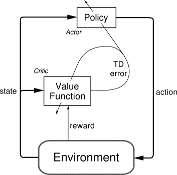
The actor-critic framework
- Remember the inconsistency (supersripts \(\pi\) and \(\pi_\phi\) for \(Q\)) in our “simple derivation” of the policy gradient formulation, \[ \nabla_\phi L_\pi(\phi) = \Expsub{\sum_{t=0}^{T-1} \nablaphi \log \piphi\agivenb{a_t}{s_t} Q^\pi(s_t, a_t)}{\tau\sim p_\phi(\tau)}? \]
- As well as Question 3. when we discussed the difference between the \(r\)-based and the \(Q\)-based versions of the policy gradient: “How can we even sample from \(\Qpiphi\) if it is not explicitly defined”?
The actor-critic framework
Actor: Neural network with parameters \(\phi\) approximates the policy: \[\pi_\phi \approx \pi.\]
Critic: Approximates \(V^\pi\) / \(Q^\pi\) / \(A^\pi\) and criticizes the actor: \[ V_\theta \approx V^\pi, \qquad Q_\theta \approx Q^\pi, \qquad A_\theta \approx A^\pi.\]
Policy gradient using, e.g., \(Q_\theta\): \[\nabla_\phi L_\pi(\phi) = \Expsub{\sum_{t=0}^{T-1} \nablaphi \log \piphi\agivenb{a_t}{s_t} Q_\theta(s_t, a_t)}{\tau\sim p_\phi(\tau)}.\]
Inspired by Sergey Levine’s CS285 lecture.
An actor-critic algorithm (1)
- Now consider the baseline version where we use the advantage function \(A^\pi\) to weight the log gradient update: \[\nabla_\phi L_\pi(\phi) = \Expsub{\sum_{t=0}^{T-1} \nablaphi \log \piphi\agivenb{a_t}{s_t} A^\pi(s_t, a_t)}{\tau\sim p_\phi(\tau)} \approx \textcolor{blue}{\frac{1}{N} \sum_{i=1}^N \cbracket{\sum_{t=0}^{T-1} \nablaphi \log\,\piphi\agivenb{a_{i,t}}{s_{i,t}} A^\pi(s_{i,t},a_{i,t})} }. \]
- Key questions:
- What should we fit? \(V^\pi\), \(Q^\pi\) or \(A^\pi\)?
- To which target should we fit?
- Recall the definition of the \(Q\)-function (with \(\gamma=1\)): \[\begin{align*} Q^\pi(s_t, a_t) &= \ExpCsub{r_{t}+ Q^\pi(s_{t+1}, a_{t+1})}{s_t,a_t}{\pi} \fragment{ = \ExpCsub{r_{t}}{s_t,a_t}{\pi} + \ExpCsub{\sum_{t'=t+1}^{T-1} r_{t'}}{s_t,a_t}{\pi}} \fragment{ = \ExpCsub{r_{t}}{s_t,a_t}{\pi} + \underbrace{\sum_{t'=t+1}^{T-1} \ExpCsub{r_{t'}}{s_t,a_t}{\pi}}_{\fragment{ =V^\pi(s_{t+1}) }} } \\ &= \ExpCsub{r_{t}}{s_t,a_t}{\pi} + \Expsub{V^\pi(s_{t+1})}{s_{t+1}\sim \pC{\cdot}{s_t,a_t}}. \end{align*}\]
- Next, we’re going to make two assumptions to turn this into an algorithm in which we can use experience.
An actor-critic algorithm (2)
Two assumptions that lead to the following approximation: \[Q^\pi(s_t, a_t) = \ExpCsub{r_{t}}{s_t,a_t}{\pi} + \Expsub{V^\pi(s_{t+1})}{s_{t+1}\sim \pC{\cdot}{s_t,a_t}} \fragment{ \approx r_{t} + V^\pi(s_{t+1}). }\]
- We just take the next reward instead of considering the expectation: \[r_{t} \approx \ExpCsub{r_{t}}{s_t,a_t}{\pi}.\] \(\circ\) This is often very reasonable.
\(\circ\) If the rewards depends deterministically on the state \(s_t\) and the action \(a_t\), then this isn’t even an approximation.
💡 In this case, people often use the notation \(r(s,a)\) to denote that the reward is a deterministic function. - Instead of considering the expectation over all next possible states, we take the value of the next state we see in our executed trajectory as a representative: \[ \Expsub{V^\pi(s_{t+1})}{s_{t+1}\sim \pC{\cdot}{s_t,a_t}} \approx V^\pi(s_{t+1}). \] \(\circ\) This is an assumption that introduces bias.
\(\circ\) But it is often still a very reasonable assumption.
\(\circ\) The strong reduction in variance justifies such a biased (but simple-to-assess) estimator.
An actor-critic algorithm (3)
- Now that we have our approximation \(Q^\pi(s_t, a_t) \approx r_{t} + V^\pi(s_{t+1})\), what to do with it?
- Let’s take another look at the advantage function \(A^\pi\): \[\fragment{ A^\pi(s_t,a_t) = Q^\pi(s_t,a_t) - V^\pi(s_t) } \fragment{ \approx r_{t} + V^\pi(s_{t+1}) - V^\pi(s_t) } \fragment{ = \hat{A}^\pi(s_t,a_t). }\]
- So let’s just approximate \(V^\pi \approx V_\theta\)!
- How do we do this? \(\Rightarrow\) We have seen this already.
\(\circ\) Monte Carlo estimates from entire trajectories: \[ L_V(\theta) = \sum_{k=1}^N \big(g_k - V_\theta(s_k)\big)^2 \fragment{ \quad \Rightarrow \quad \theta \gets \theta + \alpha\rbracket{g - V_\theta(s)} \nablatheta V_\theta(s). } \] \(\circ\) TD estimates from single-sample transitions using semi-gradients: \[\begin{align*} L_V(\theta) &= \sum_{k=1}^N \big(r_k + V_\theta(s_{k+1}) - V_\theta(s_k)\big)^2 \\ \Rightarrow \quad \theta &\gets \theta + \alpha\rbracket{r + V_\theta(s') - V_\theta(s)} \nablatheta V_\theta(s). \end{align*}\]
Algorithm: Batch actor-critic
- Sample \(\set{s_i,a_i,s'_i}_{i=1}^N\) using \(\pi_\phi\agivenb{a}{s}\).
- Fit \(V_\theta(s)\) to the sampled rewards.
- Compute advantage: \[A_\theta(s_i,a_i) = r_{i} + V_\theta(s'_i) - V_\theta(s_i).\]
- Gradient: \[\nablaphi L_\pi(\phi) \approx \frac{1}{N} \sum_{i=1}^N \nablaphi \log\pi_\phi\agivenb{a_{i}}{s_{i}} A_\theta(s_i,a_i).\]
- Gradient ascent: \(\phi \gets \phi + \alpha \nablaphi L_\pi(\phi)\).
💡 We already know what’s wrong with this approach!
\(\Rightarrow\) The target changes along with the fitted value function in step 2.
\(\Rightarrow\) Use target network \(\bar{\theta}\)?
Re-introducing the discount factor
Re-introducing the discount factor (1)
- For “simplicity”, we have disregarded the discount factor \(\gamma\) for now (i.e., \(\gamma=1\)).
- However, the derivations can be done with a discount factor in a very similar fashion.
- The changes we observe occur in two places:
- The obvious one: Our \(Q\)-function is now the discounted version: \[Q^\pi(s, a) = \ExpCsub{r + \gamma Q^\pi(s', a')}{s,a}{\pi}.\] 💡 The same obviously holds for \(V\) and \(A\).
- The subtle one: The state distribution (“state visitation probability”) changes: \[\eta_\phi(s) = \sum_{t=0}^{T-1} \gamma^t \pC{s_t = s}{\piphi}.\] 💡 The proof is quite technical and requires swapping the sum over the time steps \(t\) and the integration over \(\Sc\) in the policy gradient derivation.
- When sampling, point 2. is taken care of automatically, as we will sample according to this new distribution automatically. We thus obtain the same formulation (here using \(A^\pi\)): \[ \nabla_\phi L_\pi(\phi) = \Expsub{\sum_{t=0}^{T-1} \nablaphi \log \piphi\agivenb{a_t}{s_t} A^\pi(s_t, a_t)}{\tau\sim p_\phi(\tau)} \fragment{ \approx\textcolor{blue}{\frac{1}{N} \sum_{i=1}^N \cbracket{\sum_{t=0}^{T-1} \nablaphi \log\,\piphi\agivenb{a_{i,t}}{s_{i,t}} A^\pi(s_{i,t},a_{i,t})} }, } \] where point 1. is “hidden” in \(A^\pi\) and point 2. is “hidden” in the distribution \(\tau\sim p_\phi(\tau)\).
Re-introducing the discount factor (2)
- For a better understanding, let’s make an ad-hoc introduction of discount factors and see where this leads us.
- We start with version one of the policy gradient, i.e., Monte Carlo sampling of rewards using causality: \[ \begin{equation} \nablaphi L_\pi(\phi) \approx \frac{1}{N} \sum_{i=1}^N \cbracket{\sum_{t=0}^{T-1} \nablaphi \log\,\piphi\agivenb{a_{i,t}}{s_{i,t}}\cbracket{\sum_{t'=t}^{T-1} \textcolor{red}{\gamma^{t'-t}} r_{i,t'} }}. \label{eq:AC_discount_v1} \end{equation} \]
- Alternatively, we can start with the version without considering causality: \[ \begin{equation} \nablaphi L_\pi(\phi) \approx \frac{1}{N} \sum_{i=1}^N \cbracket{\sum_{t=0}^{T-1} \nablaphi \log\pi_\phi\agivenb{a_{i,t}}{s_{i,t}}}\cbracket{\sum_{t'=0}^{T-1}\textcolor{red}{\gamma^{t'}}r_{i,t'}}. \label{eq:AC_discount_v2} \end{equation}\] ⚡ Which one is right? There clearly is a different discount for the rewards in \(\eqref{eq:AC_discount_v1}\) and \(\eqref{eq:AC_discount_v2}\)!
- Let’s reformulate \(\eqref{eq:AC_discount_v2}\) and introduce causality again: \[\begin{align} \nablaphi L_\pi(\phi) &\approx \frac{1}{N} \sum_{i=1}^N \sum_{t=0}^{T-1} \nablaphi \log\pi_\phi\agivenb{a_{i,t}}{s_{i,t}}\cbracket{\sum_{t'=0}^{T-1}\textcolor{red}{\gamma^{t'}}r_{i,t'}} \notag \\ &= \frac{1}{N} \sum_{i=1}^N \sum_{t=0}^{T-1} \textcolor{red}{\gamma^t} \nablaphi \log\pi_\phi\agivenb{a_{i,t}}{s_{i,t}}\cbracket{\sum_{t'=t}^{T-1}\textcolor{red}{\gamma^{t' - t}}r_{i,t'}} \label{eq:AC_discount_v3} \end{align}\]
Re-introducing the discount factor (3)
\[ \underbrace{\nablaphi L_\pi(\phi) \approx \frac{1}{N} \sum_{i=1}^N \cbracket{\sum_{t=0}^{T-1} \nablaphi \log\,\piphi\agivenb{a_{i,t}}{s_{i,t}}\cbracket{\sum_{t'=t}^{T-1} \textcolor{red}{\gamma^{t'-t}} r_{i,t'} }}}_{\text{Option 1: } \eqref{eq:AC_discount_v1}} \quad\text{vs.}\quad \underbrace{\nablaphi L_\pi(\phi) \approx \frac{1}{N} \sum_{i=1}^N \sum_{t=0}^{T-1} \textcolor{red}{\gamma^t} \nablaphi \log\pi_\phi\agivenb{a_{i,t}}{s_{i,t}}\cbracket{\sum_{t'=t}^{T-1}\textcolor{red}{\gamma^{t' - t}}r_{i,t'}}}_{\text{Option 2: }\eqref{eq:AC_discount_v3}} \]
- Option 2 (Equation \(\eqref{eq:AC_discount_v3}\)) is mathematically correct.
- This makes a lot of sense. Since later rewards are less important due to the discount, later actions should also matter less!
- But: In practice, we use Option 1 (Equation \(\eqref{eq:AC_discount_v1}\))
- In many tasks, we do care about the long-term behavior.
- Additional discounting of the policy often leads to deterioration of long-term performance (e.g., in infinite-horizon problems).
Common versions of the policy gradient with discount \(\textcolor{red}{\gamma}\)
\[ \begin{align*} \text{MC reward sampling:}\quad\nabla_\phi L_\pi(\phi) &\approx \frac{1}{N} \sum_{i=1}^N \sum_{t=0}^{T-1} \nablaphi \log\pi_\phi\agivenb{a_{i,t}}{s_{i,t}}\cbracket{\sum_{t'=t}^{T-1}\textcolor{red}{\gamma^{t' - t}}r_{i,t'}} \\ \text{Advantage function:}\quad\nabla_\phi L_\pi(\phi) &\approx\frac{1}{N} \sum_{i=1}^N \Big(\sum_{t=0}^{T-1} \nablaphi \log\,\piphi\agivenb{a_{i,t}}{s_{i,t}} \underbrace{\cbracket{r_{i,t} + \textcolor{red}{\gamma} V_\theta(s_{i,t+1}) - V_\theta(s_{i,t})}}_{A_\theta(s_{i,t},a_{i,t})} \Big) \end{align*} \]
Batch and online AC with discount
Algorithm: Batch actor-critic with discount
- Sample \(\set{s_i,a_i,s'_i}_{i=1}^N\) using \(\pi_\phi\agivenb{a}{s}\).
- Fit \(V_\theta(s)\) to the sampled reward sums.
\(~\) - Compute advantages: \[A_\theta(s_i,a_i) = r_{i} + \gamma V_\theta(s'_i) - V_\theta(s_i).\]
- Gradient: \[\nablaphi L_\pi(\phi) \approx \frac{1}{N} \sum_{i=1}^N \nablaphi \log\pi_\phi\agivenb{a_{i}}{s_{i}} A_\theta(s_i,a_i).\]
- Gradient ascent: \(\phi \gets \phi + \alpha \nablaphi L_\pi(\phi)\).
Algorithm: Online actor-critic with discount
- Action \(a\sim\pi_\phi\agivenb{a}{s}\) \(\Rightarrow\) \((s,a,r,s')\).
- Update \(V_\theta(s)\) using the TD error:
\(\quad\delta = r + \gamma V_\theta(s') - V_\theta(s)\). - Compute advantage: \[A_\theta(s,a) = r + \gamma V_\theta(s') - V_\theta(s).\]
- Gradient: \[\nablaphi L_\pi(\phi) \approx \nablaphi \log\pi_\phi\agivenb{a}{s} A_\theta(s,a). \vphantom{\frac{1}{N} \sum_{i=1}^N}\]
- Gradient ascent: \(\phi \gets \phi + \alpha \nablaphi L_\pi(\phi)\).
Design decisions
Design decisions
Choice of neural networks
Now that we need to fit two functions, \(\pi_\phi\) and \(V_\theta\), how do we do this in practice?
Data collection and parallelism
- Online AC works best with batches instead of single samples.
- Option 1: parallel workers, synchronous updates.
- Option 2: parallel workers, asynchronous (but closely aligned) updates.
- Option 3: training from a replay buffer, with data collected at different times and under different policies.
- The last option requires off-policy training, even though policy gradients are originally on-policy!
Off-policy actor-critic
Online AC using off-policy data
Algorithm: Off-policy actor-critic with discount
- Action \(a\sim\pi_\phi\agivenb{a}{s}\) \(\Rightarrow\) \((s,a,r,s')\) \(\Rightarrow\) store in \(\Dc\).
- Sample batch \(\Bc \subset \Dc\) (size \(N\)) from the buffer.
- Update \(V_\theta(s)\) using the TD error:
\[\min_\theta \frac{1}{N} \sum_{i=1}^N \|\underbrace{r_i + \gamma V_\theta(s'_i) - V_\theta(s_i)}_{=\delta_i}\|_2^2.\] - Compute advantages: \[A_\theta(s_i,a_i) = r_{i} + \gamma V_\theta(s'_i) - V_\theta(s_i).\]
- Gradient: \[\nablaphi L_\pi(\phi) \approx \frac{1}{N} \sum_{i=1}^N \nablaphi \log\pi_\phi\agivenb{a_{i}}{s_{i}} A_\theta(s_i,a_i).\]
- Gradient ascent: \(\phi \gets \phi + \alpha \nablaphi L_\pi(\phi)\).
The algorithm is broken in two places! Can you spot them?
- Step 3: We are using the wrong target value.
\(V_\theta\) is on-policy and only valid for the policy \(\pi\) whose data it was trained on! - Step 5: \(\pi_\phi\agivenb{a}{s}\) does not yield the action we would have selected.
\(\Rightarrow\) To make actor-critic an off-policy algorithm, we need to fix both!
Online AC: Fixing the value function and policy
Algorithm: Off-policy actor-critic with discount
- Action \(a\sim\pi_\phi\agivenb{a}{s}\) \(\Rightarrow\) \((s,a,r,s')\) \(\Rightarrow\) store in \(\Dc\).
- Sample batch \(\Bc \subset \Dc\) (size \(N\)) from the buffer.
- Update \(Q_\theta(s)\) using the TD error:
\[\min_\theta \frac{1}{N} \sum_{i=1}^N \|\underbrace{r_i + \gamma Q_\theta(s'_i, a'_i) - Q_\theta(s_i,a_i)}_{=\delta_i}\|_2^2.\] - Compute advantages: \[A_\theta(s_i,a_i) = r_{i} + \gamma V_\theta(s'_i) - V_\theta(s_i).\]
- Gradient: \[\nablaphi L_\pi(\phi) \approx \frac{1}{N} \sum_{i=1}^N \nablaphi \log\pi_\phi\agivenb{a^{\pi_\phi}_{i}}{s_{i}} A_\theta(s_i,a_i).\]
- Gradient ascent: \(\phi \gets \phi + \alpha \nablaphi L_\pi(\phi)\).
Step 3: Use the \(Q\)-function instead of the value function!
\(\circ\) To approximate the value function of the current policy \(\pi_\phi\), we can simply sample \(a'_i\sim \pi_\phi\agivenb{\cdot}{s'_i}\).
\(\circ\) Recall (for Step 4.): \(V^\pi(s_i) = \Expsub{Q(s_i,a_i)}{a_i \sim \policy{\cdot}{s_i}}\).
Step 5: Sample the actions from the current policy, not from the replay buffer!
\(\circ\) \(a^{\pi_\phi}_{i} \sim \pi_\phi\agivenb{\cdot}{s_i}\).
Note 1: The data is still sampled from the “wrong” distribution, i.e., it is not from \(p_\phi(s)\)!
\(\Rightarrow\) There is nothing we can do about this. However, we can see this as positive, as we train a policy on a broader distribution.
Note 2: It is very common to use \(Q_\theta\) instead of \(A_\theta\) in Step 5, even though skipping the baseline leads to higher variance.
\(\Rightarrow\) Skipping the baseline is a good tradeoff, as we can simply sample additional actions (which does not require acquiring new states(!)), and thus shrink the variance arbitrarily!
Critics as baselines
Critics as state-dependent baselines
Let’s directly compare the policy gradient from the last lecture against our actor-critic procedure from today:
Policy gradient
\[ \nablaphi L_\pi(\phi) \approx \frac{1}{N} \sum_{i=1}^N \sum_{t=0}^{T-1} \nablaphi \log\pi_\phi\agivenb{a_{i,t}}{s_{i,t}}\cbracket{\cbracket{\sum_{t'=t}^{T-1}\gamma^{t'-t} r_{i,t'}} - b}\quad\]
\(\textcolor{green}{\mathbf{+}\text{ no bias}}\)
\(\textcolor{red}{\mathbf{-}\text{ high variance (single-sample estiamte)}}\)
Actor-critic
\[\nablaphi L_\pi(\phi) \approx \frac{1}{N} \sum_{i=1}^N \sum_{t=0}^{T-1} \nablaphi \log\pi_\phi\agivenb{a_{i,t}}{s_{i,t}} \cbracket{r_{i,t} + \gamma V_\theta(s_{i,t+1}) - V_\theta(s_{i,t})}\]
\(\textcolor{green}{\mathbf{+}\text{ lower variance (due to critic)}}\)
\(\textcolor{red}{\mathbf{-}\text{ not unbiased (if critic is imperfect)}}\)
Question: Can we use a critic (i.e., \(V_\theta\)) and still keep the esimator unbiased?
\(\Rightarrow\) we can make the baseline \(b\) state-dependent (proof very similar to the one from last week)!
\[ \nablaphi L_\pi(\phi) \approx \frac{1}{N} \sum_{i=1}^N \sum_{t=0}^{T-1} \nablaphi \log\pi_\phi\agivenb{a_{i,t}}{s_{i,t}}\cbracket{\cbracket{\sum_{t'=t}^{T-1}\gamma^{t'-t} r_{i,t'}} - V_\theta(s_{i,t})} \]
\(\textcolor{green}{\mathbf{+}\text{ no bias}}\)
\(\textcolor{green}{\mathbf{+}\text{ lower variance}}\)
Control variates: action dependent baselines
A natural follow-up question is: If a state-dependent baseline is stronger than a constant one, wouldn’t a baseline depending on states and actions be even better?
\(\Rightarrow\) The answer is yes! We can take the \(Q\)-function as the baseline as well. We call these approaches control variates.
(Non-bootstrapped) state-dependent baseline
\[ A_\theta(s_t,a_t) = \cbracket{\sum_{t'=t}^{T-1}\gamma^{t'-t} r_{t'}} - V_\theta(s_{t}) \]
\(\textcolor{green}{\mathbf{+}\text{ no bias}}\)
\(\textcolor{red}{\mathbf{-}\text{ higher variance (single-sample)}}\)
(Non-bootstrapped) state-action-dependent baseline
\[ A_\theta(s_t,a_t) = \cbracket{\sum_{t'=t}^{T-1}\gamma^{t'-t} r_{t'}} - Q_\theta(s_{t},a_t) \]
\(\textcolor{green}{\mathbf{+}\text{ goes to zero in expectation (if critic correct)}}\)
\(\textcolor{red}{\mathbf{-}\text{ formula is incorrect!}}\)
The term that was neglected above: \[ \nablaphi L_\pi(\phi) \approx \frac{1}{N} \sum_{i=1}^N \sum_{t=0}^{T-1} \nablaphi \log\pi_\phi\agivenb{a_{i,t}}{s_{i,t}}\cbracket{\hat{Q}_{i,t} - Q_\theta(s_{i,t}, a_{i,t})} \textcolor{blue}{+ \frac{1}{N} \sum_{i=1}^N \sum_{t=0}^{T-1} \Expsub{Q_\theta(s_{i,t},a_{t})}{a_t \sim \pi_\theta\agivenb{\cdot}{s_{i,t}}}}. \]
\(\Rightarrow\) This one is often easier to estimate. Finite \(\Ac\): compute sum! Continuous \(\Ac\): sampling actions is easy!
\(n\)-step advantage estimation
Similar to standard TD learning, we can again find some middle ground between the one-step estimate and the MC estimate: \[\begin{align*} \text{One-step TD estimate:}\qquad A_\theta(s_t,a_t) &= r_{t} + \gamma V_\theta(s_{t+1}) - V_\theta(s_t), \\ \text{MC estimate:}\qquad A_\theta(s_t,a_t) &= \cbracket{\sum_{t'=t}^{T-1}\gamma^{t'-t} r_{t'}} - V_\theta(s_{t}). \end{align*}\]
Just as before, we can simulate \(n\) steps, before bootstrapping the non-simulated piece of our trajectory: \[\qquad\qquad\qquad\qquad\text{$n$-step estimate:}\qquad A^n_\theta(s_t,a_t) = \cbracket{\sum_{t'=t}^{t+n}\gamma^{t'-t} r_{t'}} + \gamma^n V_\theta(s_{t+n}) - V_\theta(s_{t}).\]
- Near into the future (i.e., \(t'\leq t+n\)), we often have a small variance, such that a single trajectory gives us a good and unbiased estimate.
- Further into the future (i.e., \(t'>t+n\)), we likely have a higher variance, such that a single trajectory is not as helpful.
- There, using a bootstrapped estimate of the expected return (\(V_\theta(s_{t+n})\)) helps us to reduce the variance.
- \(n>1\) often works better, it is a better trade-off between bias and variance.
Generalized advantage estimation
From the \(n\)-step estimate, the next step in TD learning was to average over all possible \(n\)-step estimates \(\Rightarrow\) TD(\(\lambda\))!
- In the actor-critic setting, this is known as generalized advantage estimation (GAE): \[ A^{\mathsf{GAE}}_\theta(s_t,a_t) = \sum_{n}^\infty w_n A^n_\theta(s_t,a_t). \]

- How to weight the individual \(A^n_\theta\)?
- put more importance to earlier (low-variance) data.
- \(w_n \propto \lambda^{n-1}\) (exponentiall fall-off).
\[\begin{align*} A^{\mathsf{GAE}}_\theta(s_t,a_t) &= r_t + \gamma \Big((1-\lambda) V_\theta(s_{t+1}) + \lambda \big(r_{t+1} + \gamma \cbracket{(1-\lambda) V_\theta(s_{t+2}) + \lambda (r_{t+2} + \ldots)}\big)\Big), \\ A^{\mathsf{GAE}}_\theta(s_t,a_t) &= \sum_{t'=t}^\infty (\gamma\lambda)^{t'-t} \delta_{t'}, \qquad \text{with TD error}\quad\delta_{t'} = r_{t'} + \gamma V_\theta(s_{t'+1}) - V_\theta(s_{t'}). \end{align*}\]
\(\Rightarrow\) The discount factor serves as a means to trade off bias and variance!
References
Sutton, R. S., and A. G. Barto. 1998. Reinforcement Learning: An Introduction. MIT Press.