Deep Reinforcement Learning

Advanced Algorithms (Part II)

Prof. Dr. Sebastian Peitz

Chair of Safe Autonomous Systems, TU Dortmund

Summer term 2026

🚀 by Decker

Content

The evolution of modern RL algorithms
Part (II): Improving \(Q\)-learning
- Deterministic policy gradient
- Deep deterministic policy gradient (DDPG)
- TD3
- Soft Actor-Critic

Where are we?

Lecture contents
Chapter	Topic	Content
	Basics & tabular methods
1-5	Bandits, MDPs, Dynamic Programming, Monte Carlo, TD Learning	RL basics in finite dimensions
	Deep-learning-based methods
6	Brief introduction to deep learning	The basics for what comes next
7	Value function approximation	Value estimation with function approximation
8	Deep Q-learning	Q-learning with neural networks
9	Policy gradients	Direct optimization of the policy
10	Actor-critic algorithms	Improved policy gradients via value functions
11	Advanced algorithms (Part I): From policy gradient to PPO	The PG route to modern RL algorithms
12	Advanced algorithms (Part II): From \(Q\)-learning to Soft Actor-Critic	The AC route to modern RL algorithms
13	Exploration
	Model-Based Control
	Advanced Topics

The evolution of modern RL algorithms

(I) Policy gradient methods

Policy is explicitly parameterized and optimized directly: \[L_\pi(\phi)=\Expsub{r(\tau)}{\tau\sim p_\phi(\tau)}.\]
Gradient ascent: \(\phi \gets \phi + \alpha \nabla_\phi L_\pi(\phi)\).
Methods are typically on-policy.
Algorithms: REINFORCE \(\rightarrow\) Actor-Critic \(\rightarrow\) Natural Policy Gradient \(\rightarrow\) Trust-region policy optimization (TRPO) \(\rightarrow\) Proximal policy optimization (PPO).

(II) Value-based methods

Approximation of the \(Q\)-function:
\[Q^*(s,a) = r + \max_{a'\in\Ac}Q^*(s',a').\]
Extract implicit policy: \(\pi(s) = \arg\max_{a\in\Ac} Q^*(s,a)\).
Typically off-policy.
Algorithms: Q-learning \(\rightarrow\) DQN \(\rightarrow\) Deep deterministic policy gradient (DDPG) \(\rightarrow\) TD3 \(\rightarrow\) Soft actor-critic (SAC).

Shortcomings

High variance gradients.
Unstable policy updates.
Catastrophic performance collapse.

Shortcomings

Instability from bootstrapping.
Overestimation bias.
Maximization over actions / continuous action spaces.

Improvement strategy

How to safely update policies.

Improvement strategy

Stabilizing \(Q\)-learning with function approximation.
Solving the continuous argmax problem.

Part (II): Improving \(Q\)-learning

The problem of continuous actions in \(Q\)-learning

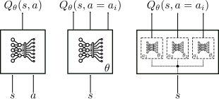
In a standard DQN, the optimal policy is implicit.
To choose the best action \(a\) in a given state \(s\), the agent evaluates the \(Q\)-values for all possible actions and picks the one that maximizes the expected return: \[\pi(s) = \arg\max_{a} Q^*(s, a)\]
Works well for discrete action spaces (e.g., Left, Right, Jump).

images/08-deep-q-learning/Model_types_action_value.svg — Types of architectures (Abdelwanis et al. 2026)

For continuous \(\Ac\) (e.g., controlling the torque of a robotic joint), we have an infinite number of possible actions.
To find the absolute maximum of the \(Q\)-function in this scenario, we can pursue two options (both very expensive):
- Discretize the action space. For instance, if we have \(7\) joints and discretize each into just \(10\) levels, we get \(10^7\) possible actions.
  \(\Rightarrow\) The “curse of dimensionality” makes this computationally impossible to solve in real-time.
- Optimization. An iterative optimization algorithm (e.g., gradient ascent) inside the environment loop to find the maximizing \(a\) before each step.

Approach: Merging DQN and Actor-Critic

Instead of maximizing over \(Q\), we introduce a function \(a = \mu_\phi(s)\) such that \(Q^*(s, \mu_\phi(s)) \approx \max_{a} Q^*(s, a)\).

Challenges:

We now have to optimize for the policy directly \(\Rightarrow\) policy gradient!
In off-policy algorithms like \(Q\)-learning, the variance becomes an even bigger problem!
- Off-policy policy gradient.
- Deterministic policies with reduced variance.

Recall: Policy gradient and actor-critic

Policy gradient theorem – formulation via reward trajectories (sampling version in blue)

\[ \nablaphi L_\pi(\phi) = \Expsub{\sum_{t=0}^{T-1} \nablaphi \log\piphi\agivenb{a_t}{s_t}\cbracket{\sum_{t'=t}^{T-1}r_{t'}}}{\tau\sim p_\phi(\tau)} \approx \textcolor{blue}{\frac{1}{N} \sum_{i=1}^N \cbracket{\sum_{t'=t}^{T-1} \nablaphi \log\,\piphi\agivenb{a_{i,t}}{s_{i,t}}\cbracket{\sum_{t'=t}^{T-1} r_{i,t'} }}}. \]

Policy gradient theorem – formulation using the \(Q\)-function and the Actor-Critic architecture

\[\nabla_\phi L_\pi(\phi) = \Expsub{\sum_{t=0}^{T-1} \nablaphi \log \piphi\agivenb{a_t}{s_t} A_\theta(s_t, a_t)}{\tau\sim p_\phi(\tau)} \approx \textcolor{blue}{\frac{1}{N} \sum_{i=1}^N \cbracket{\sum_{t=0}^{T-1} \nablaphi \log\,\piphi\agivenb{a_{i,t}}{s_{i,t}} A_\theta(s_{i,t},a_{i,t})} }. \]

Main drawbacks

High-variance gradient.
Inefficient for continuous actions, since sampling in high-dimensional settings becomes inefficient.
On-policy \(\Rightarrow\) sample-inefficient (importance sampling makes problem 1. even worse!)

Approach: Find a more sample-efficient and off-policy capable version \(\Rightarrow\) deterministic policy!

Off-policy policy gradients (1)

(Degris, White, and Sutton 2012) presented an alternative form for the off-policy policy gradient (for finite \(\Sc\) and \(\Ac\)) using an approximation. The starting point is the definition of the value function: \[\Vpiphi = \sum_{s\in\Ac} \rho_\beta(s) \sum_{a\in\Ac} \piphi\agivenb{a}{s} \Qpiphi(s,a),\] where \(\beta\) is some behavior policy and \(\rho_\beta(s) = \lim_{t\to\infty}p\agivenb{s}{s_0,\beta}\) is the limiting distribution of states when following \(\beta\).
Then, taking the gradient of \(\Vpiphi\) with respect to \(\phi\), we get (via the product rule of differentiation): \[ \nablaphi\Vpiphi = \nablaphi \rbracket{\sum_{s\in\Ac} \rho_\beta(s) \sum_{a\in\Ac} \piphi\agivenb{a}{s} \Qpiphi(s,a)} \fragment{ = \sum_{s\in\Ac} \rho_\beta(s) \sum_{a\in\Ac} \rbracket{\nablaphi\piphi\agivenb{a}{s} \Qpiphi(s,a) + \piphi\agivenb{a}{s} \nablaphi\Qpiphi(s,a)}. } \]
Ignoring the second part (i.e., \(\cancel{\piphi\agivenb{a}{s} \nablaphi\Qpiphi(s,a)}\); justification details in (Degris, White, and Sutton 2012)), we get \[ \nablaphi\Vpiphi \approx \sum_{s\in\Ac} \rho_\beta(s) \sum_{a\in\Ac} \nablaphi\piphi\agivenb{a}{s} \Qpiphi(s,a) \fragment{ = \Expsub{\sum_{a\in\Ac} \nablaphi\piphi\agivenb{a}{s} \Qpiphi(s,a)}{s\sim\rho_\beta}. } \]

Off-policy policy gradients (2)

\[ \nablaphi\Vpiphi \approx \sum_{s\in\Ac} \rho_\beta(s) \sum_{a\in\Ac} \nablaphi\piphi\agivenb{a}{s} \Qpiphi(s,a) = \Expsub{\sum_{a\in\Ac} \nablaphi\piphi\agivenb{a}{s} \Qpiphi(s,a)}{s\sim\rho_\beta}. \]

To make this off-policy w.r.t. the actions as well, we introduce importance sampling for \(\beta\): \[\begin{align*} \nablaphi\Vpiphi &\approx \sum_{s\in\Ac} \rho_\beta(s) \sum_{a\in\Ac} \textcolor{red}{\beta\agivenb{a}{s}} \underbrace{\frac{\textcolor{blue}{\piphi\agivenb{a}{s}}}{\textcolor{red}{\beta\agivenb{a}{s}}}}_{=\kappa_\phi(s,a)} \frac{\nablaphi\piphi\agivenb{a}{s}}{\textcolor{blue}{\piphi\agivenb{a}{s}}} \Qpiphi(s,a) \fragment{ = \sum_{s\in\Ac} \rho_\beta(s) \sum_{a\in\Ac} \beta\agivenb{a}{s} \kappa_\phi(s,a) \nablaphi\log\,\piphi\agivenb{a}{s} \Qpiphi(s,a) } \\ &= \Expsub{\kappa_\phi(s,a) \nablaphi\log\,\piphi\agivenb{a}{s} \Qpiphi(s,a)}{s\sim\rho_\beta,a\sim \beta\agivenb{\cdot}{s}}. \end{align*}\]
The starting point in (Silver et al. 2014) was very similar, but using continuous state and action spaces: \[\boxed{ \nablaphi\Vpiphi \approx \int_\Sc\rho_\beta(s)\int_\Ac \kappa_\phi(s,a) \nablaphi\log\,\piphi\agivenb{a}{s} \Qpiphi(s,a) \dint{a} \dint{s} = \Expsub{\kappa_\phi(s,a) \nablaphi\log\,\piphi\agivenb{a}{s} \Qpiphi(s,a)}{s\sim\rho_\beta,a\sim \beta\agivenb{\cdot}{s}}. }\]
We now have derived a simplified formula for the off-policy policy gradient.
Aside from the approximation we just made, it’s similar to the on-policy policy gradient!
However, we still suffer from the large variance issue.

Deterministic policy gradient

Deterministic off-policy policy gradients

Drop the randomness from the policy \(\mu\) such that it becomes a deterministic function: \(a = \mu_\phi(s)\).
Reformulate \(V\) via \(Q\): no need for expecations (i.e., sum / integrate over \(\Ac\)): \(V^{\mu_\phi}(s) = Q^{\mu_\phi}(s,\mu_\phi(s))\).
Deterministic: we are incapable of exploration! The theorem is only practically useful if we sample from off-policy data: \[L_\pi(\phi)= \Expsub{Q^{\mu_\phi}(s,\mu_\phi(s))}{s\sim\rho_{\beta}} = \int_\Sc \rho_{\beta}(s) Q^{\mu_\phi}(s,\mu_\phi(s)) \dint{s}. \]

Deterministic policy gradient theorem (Silver et al. 2014)

Exact version: on-policy (\(\rho_{\beta} = \rho_{\mu_\phi}\))

\[\begin{equation}\begin{aligned} \nablaphi L_\pi(\phi) &= \nablaphi\rbracket{\int_\Sc \rho_{\beta}(s) Q^{\mu_\phi}(s,\mu_\phi(s)) \dint{s}} = \int_\Sc \rho_{\beta}(s) \nablaa Q^{\mu_\phi}(s,\mu_\phi(s)) \big|_{a=\mu_\phi(s)} \nablaphi \mu_\phi(s) \dint{s} \\ &= \Expsub{\nablaa Q^{\mu_\phi}(s,\mu_\phi(s)) \big|_{a=\mu_\phi(s)} \nablaphi \mu_\phi(s)}{s\sim\rho_{\beta}}. \end{aligned} \label{eq:Adv2_dpg} \end{equation}\]

Approximate version: off-policy (\(\rho_{\beta} \neq \rho_{\mu_\phi}\), and we use the same simplification as earlier, i.e., \(\cancel{\mu_\phi\agivenb{a}{s} \nablaa Q^{\mu_\phi}(s,a)}\))

\[\begin{equation} \nablaphi L_\pi(\phi) \approx \Expsub{\nablaa Q^{\mu_\phi}(s,\mu_\phi(s)) \big|_{a=\mu_\phi(s)} \nablaphi \mu_\phi(s)}{s\sim\rho_{\beta}}.\label{eq:Adv2_dpg_approx} \end{equation}\]

💡 \(\eqref{eq:Adv2_dpg}\) is the limit case of the stochastic policy gradient theorem (i.e., \(\Var{\pi}\to 0\)) (Silver et al. 2014, Theorem 2).

On-policy deterministic actor-critic

The simplest algorithm we can derive from this: SARSA-type on-policy Actor-Critic:

Algorithm: On-policy deterministic actor-critic

Sample \(\set{s_i,a_i,r_i,s'_i,a'_i}_{i=1}^N\) using \(a = \mu_\phi(s)\).
TD error: \[\delta_i = r_i + \gamma Q_\theta(s'_i,a'_i) - Q_\theta(s_i,a_i).\]
Semi-gradient \(Q\)-function update: \[\theta \gets \theta + \alpha_\theta \frac{1}{N} \sum_{i=1}^N \delta_i \nablatheta Q_\theta(s_i,a_i).\]
Update policy \(\mu_\phi\) by sampling \(\eqref{eq:Adv2_dpg}\): \[\phi \gets \phi + \alpha \frac{1}{N} \sum_{i=1}^N \nablaa Q_\theta(s_i,a_i) \nablaphi \mu_\phi(s_i).\]

Summary of the concept

To update a deterministic policy off-policy, your algorithm does this for a batch of states from the replay buffer:

Pass state \(s\) into the actor: \(a = \mu_\phi(s)\).
Pass \(s\) and \(a\) into the critic network \(Q_\theta(s, a)\).
Compute how the critic’s output changes with respect to that action (\(\nabla_a Q\)).
Compute how the actor’s weights change to produce that action change (\(\nablaphi \mu_\phi\)).
Multiply them together to update the actor.

Deep deterministic policy gradient (DDPG)

Problems with vanilla DPG

The original algorithm assumed:

tabular / linear approximators (“Compatible Function Approximation” in (Silver et al. 2014)),
stable \(Q\) estimation.

When neural networks are used, several problems appear:

Bootstrapping instability.
Correlated samples from trajectories.
Targets change too quickly.
Poor exploration due to deterministic policy.

Deep deterministic policy gradient (DDPG) (Lillicrap et al. 2016)

addresses these by importing techniques from Deep Q-Networks (DQN).

Core components:

Actor network \(\mu_\phi(s)\)
Critic network \(Q_\theta(s,a)\)
Target actor \(\mu_{\bar{\phi}}\)
Target critic \(Q_{\bar{\theta}}\)
Replay buffer

The DDPG algorithm

Interact: Sample \(\set{s_t,a_t,r_t,s_{t+1}}\) using \(a_t=\mu_\phi(s_t)\) (💡 plus noise for exploration!) and store in the replay buffer \(\Dc\).
Sample: Draw random mini-batch of \(N\) transitions: \(\Bc\subset\Dc\).
Update critic: Calculate the target \(y_i\) using the target networks (💡 Optimal action \(\mu_{\bar{\phi}}(s)\) \(\Rightarrow\) \(Q\)-learning!): \[y_i = r_i + \gamma Q_{\bar{\theta}}(s_{i+1}, \mu_{\bar{\phi}}(s_{i+1})).\] The current critic is updated by minimizing the Bellman error: \[L_Q(\theta) = \frac{1}{N}\sum_{i} \cbracket{y_i - Q_\theta(s_i, a_i)}^2, \qquad \theta \gets \theta + \alpha_\theta \frac{2}{N} \sum_{i=1}^N \cbracket{y_i - Q_\theta(s_i, a_i)} \nablatheta Q_\theta(s_i,a_i).\]

Update actor: The current actor is updated using the sampled deterministic policy gradient (Eq. \(\eqref{eq:Adv2_dpg}\)): \[\phi \gets \phi + \alpha \frac{1}{N} \sum_{i=1}^N \nablaa Q_\theta(s_i,a)\Big|_{a=\mu_\phi(s_i)} \nablaphi \mu_\phi(s_i).\]
Soft updates: Incremental target updates (\(\bar{\phi}\) / \(\bar{\theta}\)).

The four main changes over DPG

Integration of deep neural networks (CNNs)
Introduction of the replay buffer

Larger datasets to train from.
Allows for i.i.d. sampling / breaks the temporal correlation of data.

Explicit action noise for exploration

Deterministic actor in DPG: it cannot explore on its own.
DDPG adds an explicit random process \(\Nc\) directly to the action selection during environment interaction.
The original paper utilized Ornstein-Uhlenbeck noise, which creates temporally correlated, mean-reverting patterns that mimic inertial drift.

Transition to “soft updates” for target networks

In DQN, target network weights are periodically copied exactly from the online network every few thousand steps.
For continuous actor-critic configurations, hard updates changed the value landscape too abruptly.
Instead: soft update, where target networks track the online networks smoothly at every single training step using an interpolation factor \(\tau \ll 1\) (e.g., \(\tau = 0.001\)): \[\bar{\theta} \leftarrow \tau \theta + (1 - \tau)\bar{\theta}, \qquad \bar{\phi} \leftarrow \tau \phi + (1 - \tau)\bar{\phi}.\] \(\Rightarrow\) targets change slowly, providing an unmoving baseline that stabilizes the deep network’s gradients.
We have seen this before under Polyak averaging.

images/08-deep-q-learning/Polyak-averaging.svg

Twin Delayed Deep Deterministic Policy Gradient (TD3)

DDPG works on many tasks, but is highly sensitive to hyperparameters as well as other randomness (e.g., the sampling).
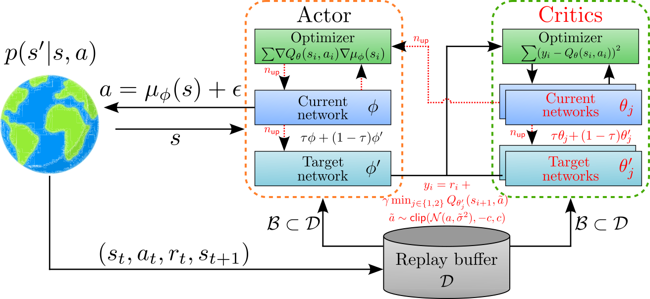
\(\Rightarrow\) In TD3 (Fujimoto, Hoof, and Meger 2018), three main issues were identified and addressed:

1. Maximization bias \(\Rightarrow\) clipped double \(Q\)-learning

Because the target uses a greedy step over actions \(a = \mu_\phi(s)\), errors accumulate \(\Rightarrow\) large overestimation bias.
Two independent critics (\(Q_{\theta_1}\) / \(Q_{\theta_2}\) and targets \(Q_{\bar{\theta}_1}\) / \(Q_{\bar{\theta}_2}\)), using the minimum of their predictions to compute the target: \[y = r + \gamma \min_{i=1,2} Q_{\bar{\theta}_i}(s', \mu_{\bar{\phi}}(s'))\]

2. Inaccurate critic \(\Rightarrow\) delayed policy updates

If the critic is highly inaccurate, updating the actor based on its gradients is counterproductive.
Delaying the policy updates ensures the critic has reached a reliable value before the actor uses it.

\(~\Rightarrow\) Update actor (\(\phi\)) and targets (\(\bar{\phi}\), \(\bar{\theta}_1\), \(\bar{\theta}_2\)) less frequently than critics (\(\theta_1\), \(\theta_2\)), e.g., every \(n_\mathsf{up}=2\) steps.

3. Exploitation of artifacts in \(Q\) \(\Rightarrow\) target action smoothing

Deterministic policies are prone to exploiting sharp peaks or artifacts in the \(Q\)-function.
Adding noise smooths out the value landscape, ensuring that similar actions yield similar values.

\(~\Rightarrow\) TD3 adds a small amount of clipped noise (clipping constant \(c\)) to the target action before feeding it into the target critic: \[\tilde{a} = \mu_{\bar{\phi}}(s) + \epsilon, \quad \epsilon \sim \mathsf{clip}(\mathcal{N}(0, \tilde{\sigma}^2), -c, c).\]

The TD3 algorithm

Interact: Sample \(\set{s_t,a_t,r_t,s_{t+1}}\) using \(a_t=\mu_\phi(s_t) + \epsilon\) (\(\epsilon\sim\Normal{0}{\sigma^2}\)) and store in the replay buffer \(\Dc\).
Sample: Draw random mini-batch of \(N\) transitions: \(\Bc\subset\Dc\).
Update critic: Calculate targets \(y_i\) by minimizing over two target networks (💡 the Twin): \[y_i = r_i + \gamma \min_{j\in\set{1,2}} Q_{\bar{\theta}_j}(s_{i+1}, \tilde{a}_{i+1}), \qquad\text{with \textcolor{red}{noisy action} }\tilde{a}_{i+1}=\mu_{\bar{\phi}}(s_{i+1}) + \epsilon, \quad\epsilon \sim \mathsf{clip}(\mathcal{N}(0, \tilde{\sigma}^2), -c, c).\] The two critics are updated by minimizing the Bellman errors: \[L_Q(\theta_j) = \frac{1}{N}\sum_{i} \cbracket{y_i - Q_{\theta_j}(s_i, a_i)}^2, \qquad \theta_j \gets \theta_j + \alpha_\theta \frac{2}{N} \sum_{i=1}^N \cbracket{y_i - Q_{\theta_j}(s_i, a_i)} \nablatheta Q_{\theta_j}(s_i,a_i).\]

Perform next steps only every \(n_\mathsf{up}\) steps: (💡 the Delayed):

Update actor: \[\phi \gets \phi + \alpha \frac{1}{N} \sum_{i=1}^N \nablaa Q_{\textcolor{red}{\theta_1}}(s_i,a)\Big|_{a=\mu_\phi(s_i)} \nablaphi \mu_\phi(s_i).\]
Soft updates: Incremental target updates (\(\bar{\phi}\) / \(\textcolor{red}{\bar{\theta}_1}\) / \(\textcolor{red}{\bar{\theta}_2}\)).

images/11-advanced/TD3_numbered.svg

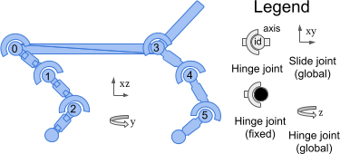
Example: Half-Cheetah

Half Cheetah from the MuJoCo library.

\(\Sc\): 17 states, \(\Ac\): 6 actions.
Reward: Forward-Cost - Control-Cost.

Results: TRPO vs. PPO vs. TD3 (from the RL Baselines3 Zoo)

TRPO

PPO

TD3

Soft actor-critic (SAC)

Introducing entropy

The limitations of both DDPG and TD3 are still quite severe.

Overestimation bias (DDPG).
Hyperparameter sensitivity (DDPG).

Lack of exploration (both).
Sample inefficiency due to Local Optima (both).

Entropy (defined by Claude Shannon in 1948).

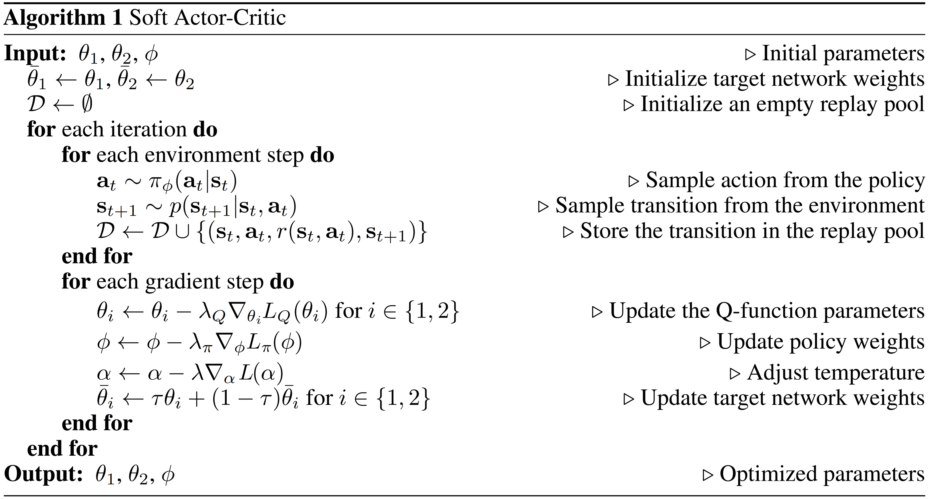
SAC (Haarnoja, Zhou, Abbeel, et al. 2018) introduces an entropy term in the loss function. \[\begin{equation} L_\pi(\phi)=\sum_{t=0}^{T-1}\gamma^t \Expsub{r_t + \alpha \Hc(\piphi\agivenb{\cdot}{s_t})}{(s_t,a_t)\sim\rho_{\piphi}}, \quad\text{where}~ \Hc(\piphi\agivenb{\cdot}{s}) = \Expsub{-\log \piphi\agivenb{a}{s}}{a \sim \piphi\agivenb{\cdot}{s}}. \label{eq:Adv2_entropy_objective} \end{equation}\]
It describes the level of uncertainty (or unpredictability) of a random variable.
\(\Hc(\piphi\agivenb{\cdot}{s_t})\) is the entropy, measuring how unpredictable the policy is.
High entropy \(\Rightarrow\) the agent explores widely.\(\quad\) Low entropy \(\Rightarrow\) it is focused on a few actions.
The temperature \(\alpha\) (a tunig parameter) determines how much the agent values exploration vs. exploitation.
By rewarding the agent for being unpredictable, it
- naturally explores the entire environment,
- prevents the policy from collapsing into a single repetitive action too early,
- becomes more robust to environment changes.

The entropy objective and value function

Let’s look at the definition of the entropy in Eq. \(\eqref{eq:Adv2_entropy_objective}\): \[ \Hc(\pi\agivenb{\cdot}{s}) = \Expsub{-\log \pias}{a \sim \pi\agivenb{\cdot}{s}}.\]
Now let’s expand the value function in the RL objective \(\eqref{eq:Adv2_entropy_objective}\): \[\begin{align} V^\pi(s_t) &= \Expsub{\sum_{k=0}^{\infty} \gamma^k \cbracket{r_{t+k} + \alpha \Hc(\piphi\agivenb{\cdot}{s_{t+k}})}}{(s_t,a_t)\sim\rho_{\piphi}} \notag \\ &= \Expsub{r_{t} + \alpha \Hc(\piphi\agivenb{\cdot}{s_{t}})}{a_t\sim \pi\agivenb{\cdot}{s_t}} + \Expsub{\sum_{k=1}^{\infty} \gamma^k \cbracket{r_{t+k} + \alpha \Hc(\piphi\agivenb{\cdot}{s_{t+1}})}}{(s_t,a_t)\sim\rho_{\piphi}} \notag \\ &= \Expsub{r_{t} - \alpha \log \pi\agivenb{a_t}{s_t}}{a_t\sim \pi\agivenb{\cdot}{s_t}} + \gamma \Expsub{V^\pi(s_{t+1})}{s_{t+1}\sim p(s_{t+1})} \label{eq:Adv2_entropy_value} \end{align}\]

Deriving the entropy \(Q\)-function

As \(a_t\) is already chosen, there is no entropy for the immediate action (its probability is one after selection).
The entropy only applies to future actions.
Therefore, we define the soft \(Q\)-function as the immediate reward plus the discounted future soft values: \[\begin{equation} Q^\pi(s_t, a_t) = r_t + \gamma \Expsub{V^\pi(s_{t+1})}{s_{t+1} \sim p(s_{t+1})}. \label{eq:Adv2_entropy_Q}\end{equation}\]
Substitute \(\eqref{eq:Adv2_entropy_Q}\) into \(\eqref{eq:Adv2_entropy_value}\): \[ V^\pi(s_t) = \Expsubbig{\underbrace{r_{t} + \gamma \Expsub{V^\pi(s_{t+1})}{s_{t+1}\sim p(s_{t+1})}}_{=Q^\pi(s_t, a_t)~\text{(Eq. \eqref{eq:Adv2_entropy_Q})}} - \alpha \log \pi\agivenb{a_t}{s_t}}{a_t\sim \pi\agivenb{\cdot}{s_t}} = \Expsubbig{Q^\pi(s_t, a_t) - \alpha \log \pi\agivenb{a_t}{s_t}}{a_t\sim \pi\agivenb{\cdot}{s_t}}. \]
We thereby obtain the soft Bellman equation: \[\begin{equation} Q^\pi(s_t, a_t) = r_t + \gamma \Expsub{Q^\pi(s_{t+1}, a_{t+1}) - \alpha \log \pi(a_{t+1} | s_{t+1})}{(s_{t+1}, a_{t+1}) \sim \rho_\piphi}. \label{eq:Adv2_entropy_soft_Bellman} \end{equation}\]

Soft actor-critic: ingredients

Neural networks

An actor network \(\piphi\).
Two critic networks \(Q_{\theta_1}\) / \(Q_{\theta_2}\) and their respective target networks \(Q_{\bar \theta_1}\) / \(Q_{\bar \theta_2}\).

Objective functions

Critic updates (based on \(\eqref{eq:Adv2_entropy_soft_Bellman}\)): \[\begin{equation} L_Q(\theta_j) = \frac{1}{N} \sum_{i=1}^N \cbracket{y_i - Q_{\theta_j}(s_i, a_i)}^2 \quad \text{with target}\quad y_i = r_i + \gamma \cbracket{\min_{j=1,2} Q_{\bar\theta_j}(s_i', a_i') - \alpha \log \piphi\agivenb{a_i'}{s_i'}}. \label{eq:Adv2_SAC_loss_Q} \end{equation}\]
Actor updates (where we either use \(\theta_1\) or the minimum of both critics): \[\begin{equation} L_\pi(\phi) = \frac{1}{N} \sum_{i=1}^N \cbracket{\alpha \log \piphi\agivenb{a_i}{s_i} - Q_{\theta_1}(s_i,a_i)}. \label{eq:Adv2_SAC_loss_pi} \end{equation}\]
Temperature updates: \[\begin{equation} L(\alpha) = \frac{1}{N} \sum_{i=1}^N \cbracket{-\alpha \log \piphi\agivenb{a_i}{s_i} - \alpha \bar \Hc}. \label{eq:Adv2_SAC_loss_temp} \end{equation}\]

The actor objective (1)

To see how we arrived at the objective \(L_\pi\), we start from defining a target distribution over the actions.
One way to represent the target distribution: probability of choosing an action proportional to its exponential soft \(Q\)-value: \[\pi_{\mathsf{target}}\agivenb{a}{s} = \frac{\exp\cbracket{\frac{Q^\pi(s, a)}{\alpha}}}{Z^\pi(s)} \qquad \text{with}\quad Z^\pi(s) = \int \exp\cbracket{\frac{Q^\pi(s, a)}{\alpha}}\dint{a}.\]
This is known as the Boltzmann distribution (or Gibbs distribution), with two useful properties:
- Actions with higher \(Q\)-values have exponentially higher probabilities of being chosen.
- The temperature \(\alpha\) scales how pronounced these differences are. If \(\alpha \to 0\), it becomes a sharp peak at the max \(Q\)-value (greedy). If \(\alpha \to \infty\), it becomes a uniform distribution (pure random exploration).
The SAC goal is thus to push the policy towards the target distribution: \[\begin{align*} L_\pi(\phi) &= \KLdivavg{\piphi}{\pi_{\mathsf{target}}} = \Expsub{\log\cbracket{\frac{\piphi\agivenb{a}{s}}{\pi_{\mathsf{target}}\agivenb{a}{s}}}}{s\sim \rho, a\sim\piphi} \fragment{ = \Expsub{\log\cbracket{\piphi\agivenb{a}{s}} - \log\cbracket{\frac{\exp\cbracket{\frac{Q^\pi(s, a)}{\alpha}}}{Z^\pi(s)}}}{s\sim \rho, a\sim\piphi} }\\ &= \Expsub{\log\cbracket{\piphi\agivenb{a}{s}} - \log\cbracket{\exp\cbracket{\frac{Q^\pi(s, a)}{\alpha}}} + \log\cbracket{Z^\pi(s)}}{s\sim \rho, a\sim\piphi} \\ &= \Expsub{\log\cbracket{\piphi\agivenb{a}{s}} - \frac{Q^\pi(s, a)}{\alpha} + \log\cbracket{Z^\pi(s)}}{s\sim \rho, a\sim\piphi}. \end{align*}\]

The actor objective (2)

\[L_\pi(\phi) = \Expsub{\log\cbracket{\piphi\agivenb{a}{s}} - \frac{Q^\pi(s, a)}{\alpha} + \log\cbracket{Z^\pi(s)}}{s\sim \rho, a\sim\piphi}.\]

Multiplying by \(\alpha\) and neglecting the policy-independent \(Z\)-term don’t change the minimizer \(\Rightarrow\) Sampling version: \[\begin{equation} L_\pi(\phi) = \frac{1}{N} \sum_{i=1}^N \cbracket{\alpha \log \piphi\agivenb{a_i}{s_i} - Q_{\theta_1}(s_i,a_i)}. \tag{\ref{eq:Adv2_SAC_loss_pi}} \end{equation}\]

Soft Policy Improvement Theorem (Haarnoja, Zhou, Hartikainen, et al. 2018, Lemma 2)

If we define: \[\subnew{\pi} = \arg\min_{\pi'} \KLdiv{ \pi'\agivenb{\cdot}{s}}{\frac{\exp\left(\frac{Q^{\subold{\pi}}\agivenb{\cdot}{s}}{\alpha}\right)}{Z^{\subold{\pi}}(s)}},\] then the soft \(Q\)-value of the new policy is guaranteed to be monotonically greater than or equal to the old one for all \((s,a)\): \[Q^{\subnew{\pi}}(s, a) \geq Q^{\subold{\pi}}(s, a) \quad \forall (s,a).\]

The reparametrization trick

Because the action \(a\) is sampled from a stochastic policy \(\piphi\), we cannot backpropagate gradients from the critic through the action to the actor directly.
Fix in SAC \(\Rightarrow\) the reparameterization trick: We express the action as a deterministic function of the state and an independent noise vector \(\epsilon\): \[a = f_\phi(\epsilon; s) = \tanh(\mu_\phi(s) + \sigma_\phi(s) \odot \epsilon), \quad \epsilon \sim \Normal{0}{I}.\]
- The neural network deterministically outputs the mean \(\mu_\phi(s)\) and standard deviation \(\sigma_\phi(s)\).
- The \(\tanh\) function bounds the actions to a valid range (e.g., \([-1, 1]\)).
Rewriting the objective with this reparameterization allows us to rewrite the expectation over the noise \(\epsilon\): \[L_\pi(\phi) = \Expsub{\alpha \log \piphi\agivenb{f_\phi(\epsilon; s)}{s} - Q_{\phi_1}(s, f_\phi(\epsilon; s))}{s \sim \Dc, \epsilon \sim \Nc}.\]
Now, the gradient with respect to \(\phi\) can flow through \(f_\phi\).
Analogous to earlier (deterministic) policy gradients, we obtain (Haarnoja, Zhou, Hartikainen, et al. 2018): \[\nablaphi L_\pi(\phi) = \Expsub{\nablaphi \alpha \log \piphi\agivenb{a}{s} + \cbracket{\alpha \nabla_a \log \piphi\agivenb{a}{s} - \nabla_a Q_{\theta_1}(s, a)} \nablaphi f_\phi(\epsilon; s)}{s \sim \mathcal{D}, \epsilon \sim \mathcal{N}}.\]

The temperature objective

To prevent hand-tuning the entropy coefficient \(\alpha\), SAC treats it as a constrained optimization problem: maximize expected reward subject to a minimum entropy constraint \(\bar{\mathcal{H}}\) (More details in (Haarnoja, Zhou, Hartikainen, et al. 2018, Chapter 5)).
SAC tunes \(\alpha\) to match a target entropy \(\bar{\Hc}\) (usually chosen as the negative action space dimension \((-m)\)).
The dual objective function minimized to find the optimal scaling parameter \(\alpha\) is: \[\begin{equation} L(\alpha) = \Expsub{-\alpha \log \pi_\theta(a|s) - \alpha \bar{\mathcal{H}}}{s \sim \mathcal{D}, a \sim \pi_\theta} = \Expsub{-\alpha( \log \pi_\theta(a|s) + \bar{\mathcal{H}})}{s \sim \mathcal{D}, a \sim \pi_\theta}. \tag{\ref{eq:Adv2_SAC_loss_temp}} \end{equation}\]
Since \(L(\alpha)\) is linear with respect to \(\alpha\), taking the derivative is straightforward: \[\nabla_\alpha L(\alpha) = -\Expsub{( \log \pi_\theta(a|s) + \bar{\mathcal{H}})}{s \sim \mathcal{D}, a \sim \pi_\theta}.\]

Intuition of the \(\alpha\) Gradient

If the current policy’s entropy is low, then \(-\log \piphi\agivenb{a}{s}\) will be a large positive number.
- If \(-\log \piphi\agivenb{a}{s} > \bar{\Hc}\), the gradient is negative, which causes \(\alpha\) to increase during gradient descent (\(\alpha \gets \alpha - \lambda \nabla_\alpha L(\alpha)\)).
- Higher \(\alpha\) forces the actor to prioritize exploration.
If the policy’s entropy is high, the gradient becomes positive, causing \(\alpha\) to decrease, shifting priorities toward maximizing standard environmental rewards.

The SAC algorithm

images/11-advanced/SAC_algorithm.png — (Haarnoja, Zhou, Hartikainen, et al. 2018)

Example: Half-Cheetah

Half Cheetah from the MuJoCo library.

\(\Sc\): 17 states, \(\Ac\): 6 actions.
Reward: Forward-Cost - Control-Cost.

Results: TRPO vs. PPO vs. TD3 vs. SAC (from the RL Baselines3 Zoo)

TRPO

PPO

TD3

SAC

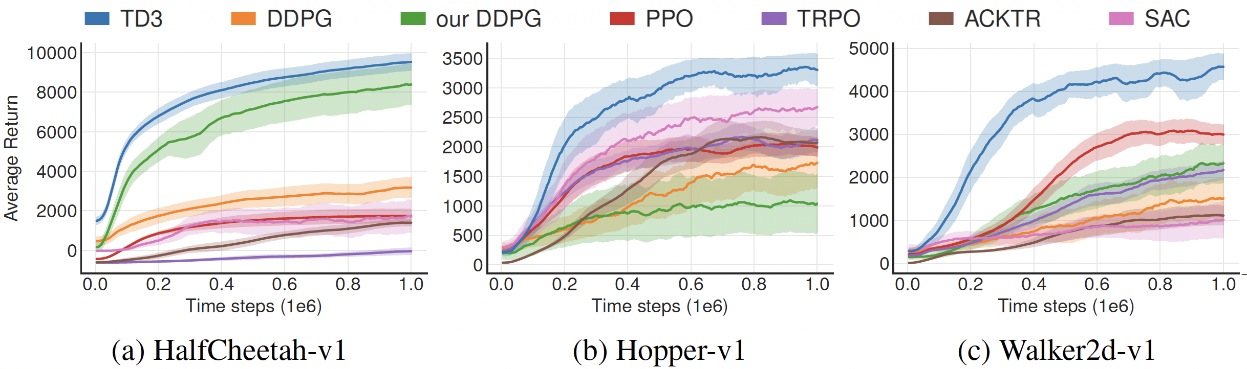
Example: Some MuJoCo environments

images/11-advanced/SAC_MuJoCo.png — Source: (Fujimoto, Hoof, and Meger 2018, Figure 5).

Half cheetah (SAC).

Hopper (SAC).

Walker 2D (SAC).

💡 Trained models from StableBaselines3.

Notes

The SAC results reported in the TD3 paper (Fujimoto, Hoof, and Meger 2018) (see left) are worse than the TD3 results.
Reason: there were two versions of SAC in quick succession.
1. The now-standard that we have discussed (Haarnoja, Zhou, Hartikainen, et al. 2018). It also considered some ideas from the TD3 paper such as twin \(Q\) networks to avoid maximization bias.
2. The original one (Haarnoja, Zhou, Abbeel, et al. 2018) went out of fashion quickly, but appeared around the same time as TD3. It is thus likely that (Fujimoto, Hoof, and Meger 2018) compared against this version.

Comparison of the algorithms we have seen in part II

Actor-Critic.
DDPG \(\Rightarrow\) variance reduction via deterministic policy.
TD3 \(\Rightarrow\) addresses maximization bias (twin networks) and inaccurate critics (via delayed updates).
SAC \(\Rightarrow\) entropy objective for natural exploration

Feature	DDPG	TD3	SAC
Policy Type	Deterministic	Deterministic	Stochastic
Exploration	Additive Noise (e.g., OU Noise)	Additive Noise (Gaussian)	Intrinsic (Entropy Maximization)
Q-Overestimation Cure	None	Clipped Double-Q	Clipped Double-Q
Sensitivity to Hyperparameters	Extremely High	High	Low (Very Stable)
Sample Efficiency	Moderate	Good	Excellent

References

Abdelwanis, Ali, Barnabas Haucke-Korber, Darius Jakobeit, Wilhelm Kirchgässner, Marvin Meyer, Maximilian Schenke, Hendrik Vater, Oliver Wallscheid, and Daniel Weber. 2026. “Reinforcement Learning: A Comprehensive Open-Source Course.” Journal of Open Source Education 9 (97). The Open Journal: 306. doi:10.21105/jose.00306.

Degris, Thomas, Martha White, and Richard S. Sutton. 2012. “Off-Policy Actor-Critic.” In International Conference on Machine Learning.

Fujimoto, Scott, Herke van Hoof, and David Meger. 2018. “Addressing Function Approximation Error in Actor-Critic Methods.” In Proceedings of the 35th International Conference on Machine Learning, edited by Jennifer Dy and Andreas Krause, 80:1587–96. Proceedings of Machine Learning Research. PMLR.

Haarnoja, Tuomas, Aurick Zhou, Pieter Abbeel, and Sergey Levine. 2018. “Soft Actor-Critic: Off-Policy Maximum Entropy Deep Reinforcement Learning with a Stochastic Actor.” In Proceedings of the 35th International Conference on Machine Learning, edited by Jennifer Dy and Andreas Krause, 80:1861–70. Proceedings of Machine Learning Research. PMLR.

Haarnoja, Tuomas, Aurick Zhou, Kristian Hartikainen, George Tucker, Sehoon Ha, Jie Tan, Vikash Kumar, et al. 2018. “Soft Actor-Critic Algorithms and Applications.” arXiv:1812.05905.

Lillicrap, Timothy P., Jonathan J. Hunt, Alexander Pritzel, Nicolas Heess, Tom Erez, Yuval Tassa, David Silver, and Daan Wierstra. 2016. “Continuous Control with Deep Reinforcement Learning.” In International Conference on Learning Representations (ICLR).

Silver, David, Guy Lever, Nicolas Heess, Thomas Degris, Daan Wierstra, and Martin Riedmiller. 2014. “Deterministic Policy Gradient Algorithms.” In International Conference on Machine Learning, edited by Eric P. Xing and Tony Jebara, 32:387–95. Proceedings of Machine Learning Research 1. Bejing, China: PMLR.