Deep Reinforcement Learning

Exploration

Prof. Dr. Sebastian Peitz

Chair of Safe Autonomous Systems, TU Dortmund

Summer term 2026

🚀 by Decker

Content

Content

  • Recap
    • Exploration-exploitation dilemma
    • Multi-armed bandits
  • Advanced exploration methods for tabular approaches
    • Upper confidence bounds
    • Thompson sampling
    • Information gain
  • Exploration in continuous spaces
    • Novelty-driven exploration: intrinsic motivation
    • The counting problem & pseudo-counts
    • Curiosity-driven exploration
    • Exploration via posterior sampling
    • Random network distillation

Where are we?

Lecture contents
Chapter Topic Content
Basics & tabular methods
1-5 Bandits, MDPs, Dynamic Programming, Monte Carlo, TD Learning RL basics in finite dimensions
Deep-learning-based methods
6 Brief introduction to deep learning The basics for what comes next
7 Value function approximation Value estimation with function approximation
8 Deep Q-learning Q-learning with neural networks
9 Policy gradients Direct optimization of the policy
10 Actor-critic algorithms Improved policy gradients via value functions
11 Advanced algorithms (Part I): From policy gradient to PPO The PG route to modern RL algorithms
12 Advanced algorithms (Part II): From \(Q\)-learning to Soft Actor-Critic The AC route to modern RL algorithms
13 Exploration How to explore in complex scenarios
Model-Based Control
Advanced Topics

Recap

Exploration-exploitation dilemma

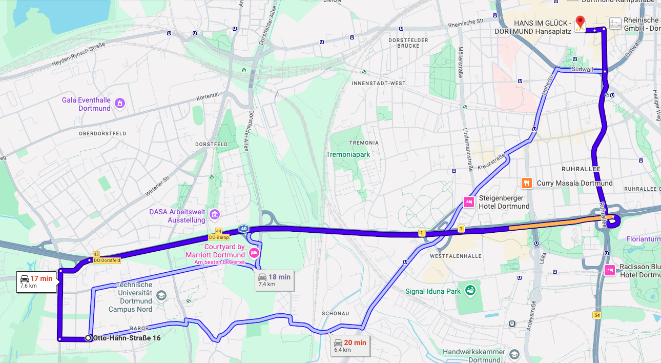
images/01-multi-armed-bandits/MapsDortmund.png
Google Maps (go here for the live version; do you get the same numbers?)
  • Let’s assume we do not have access to travel time estimates
  • Which route should I take to minimize my travel time?
  • Let’s say we can guess the time of one route fairly well
    • should we always take this one?
    • or try something else and see if we can get better?
  • This is known as the exploration-exploitation dilemma
  • The route pickig problem is one example of a multi-armed bandit

Multi-armed bandits

  • Let us assume that we have a slot machine and we repeatedly can choose between \(k\) different actions
  • After each choice \(a_t\) you receive a numerical reward \(r_t\) chosen from a stationary probability distribution\(^*\)
  • Objective: maximize the expected total reward over some time period (e.g., over 1000 action selections, or time steps)
  • We refer to this as the value: \[ q(a) = \ExpC{r_t}{a_t=a} \]
  • If we knew \(q(a)\), then it would be easy to choose!
  • Instead, we have to rely on estimates \(Q_t(a)\) which we can iteratively update based on past experience

images/01-multi-armed-bandits/multi-armed-bandit.png
A multi-armed bandit (Ferreira, Schubert, and Scotti 2024)

A simple bandit algorithm

# Initialization
for i in range(k):
  Q(a) = 0
  N(a) = 0

# Run forever
while(True):

  # exploration versus exploitation
  if rand() > epsilon:
    a = argmax(Q)        # exploitation
  else:
    a = randint(k)       # exploration

  r = bandit(a)

  # Error correction towards target r 
  N(a) = N(a) + 1
  Q(a) = Q(a) + (1/N(a)) * (r - Q(a))
A simple version of the \(\epsilon\) greedy bandit.
  • \(\epsilon\)-greey is a very simple approach to achieve (local) exploration!
  • Another approach: optimistic initial values.
    • For \(q(a) \sim \Normal{1}{0}\), an initial guess of \(Q_1(a)=5\) is certainly unrealistically high.
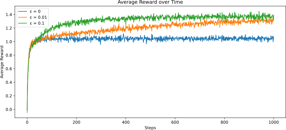
images/01-multi-armed-bandits/mab-rewards.svg
2026-03-23T23:19:47.331537 image/svg+xml Matplotlib v3.10.7, https://matplotlib.org/

Exploration in Soft Actor Critic

\[L_\pi(\phi)=\sum_{t=0}^{T-1}\gamma^t \Expsub{r_t + \alpha \Hc(\piphi\agivenb{\cdot}{s_t})}{(s_t,a_t)\sim\rho_{\piphi}}~\text{with entropy}~\Hc(\piphi\agivenb{\cdot}{s}) = \Expsub{-\log \piphi\agivenb{a}{s}}{a \sim \piphi\agivenb{\cdot}{s}}\]
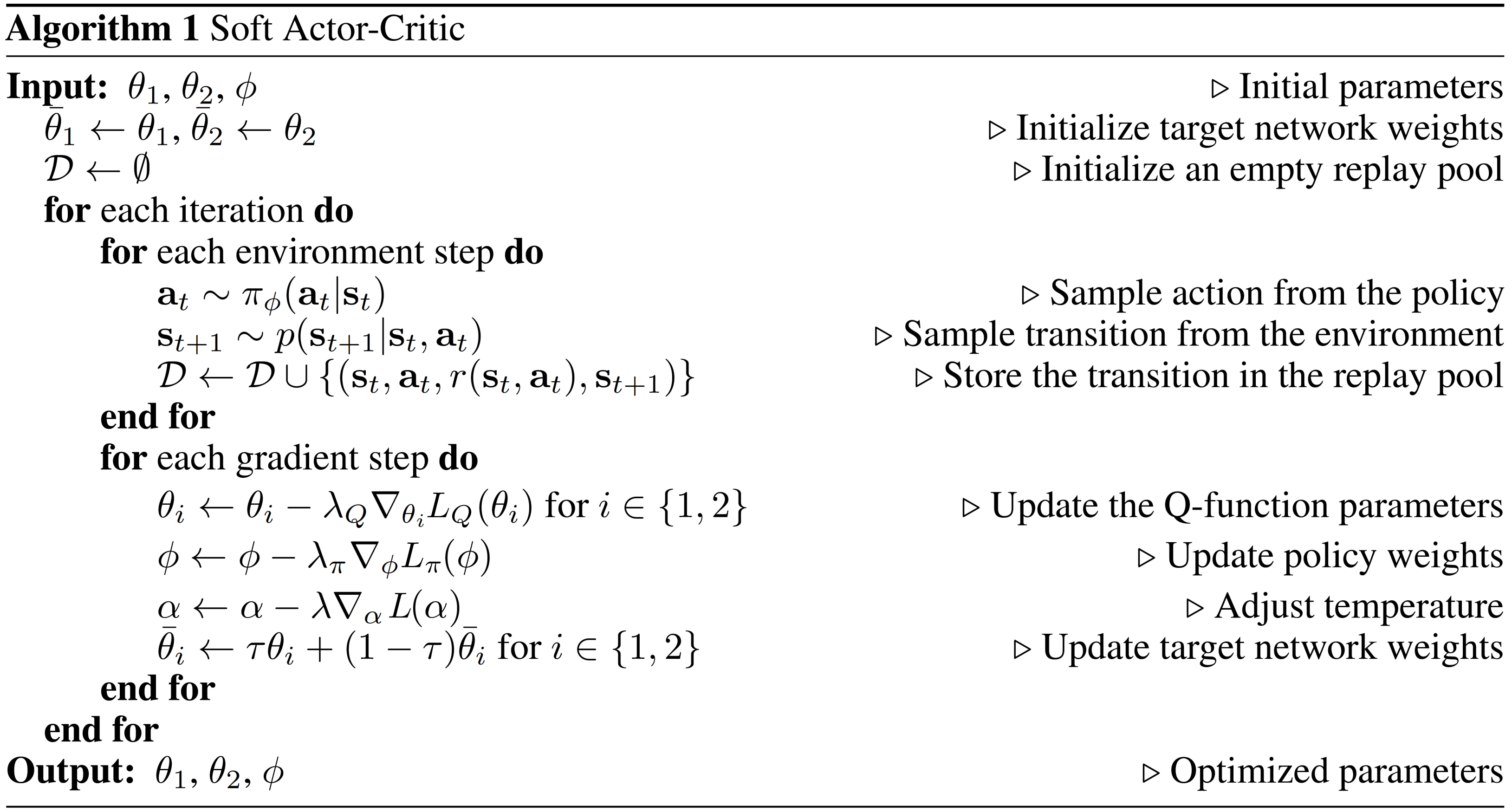
Half cheetah (SAC). Hopper (SAC).

The challenge with exploration

This is “easy”

videos/08-deep-q-learning/DQN_Pong/rl_model_2000000_steps.gif
Pong.

This is very hard!

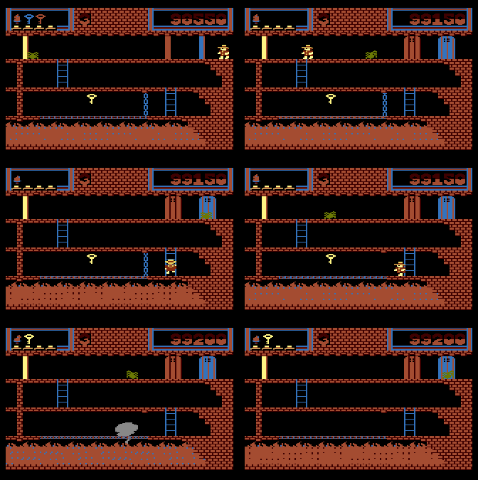
images/13-exploration/Montezumas-Revenge.gif
Montezuma’s revenge.


  • Getting key = reward
  • Opening door = reward
  • Dying = nothing (is it good? bad?)
  • Finishing the game only weakly correlates with rewarding events
  • We know what to do because we understand the concept!

Another example: The game of Mao

images/13-exploration/cards.jpg
A deck of cards for playing Mao.
  • Goal: Get rid of all the cards!
  • “The only rule you may be told is this one”.
  • There’s a penalty for breaking a rule \(\Rightarrow\) Draw another card.
  • You can only discover rules through trial and error.
  • The rules don’t always make sense to you.


Temporally extended tasks like Montezuma’s revenge become increasingly difficult based on

  • How extended the task is.
  • How little you know about the rules.

âť“ Imagine your goal was winning 50 games of Mao in a row, without knowing the rules!

Advanced exploration methods for tabular approaches

Upper confidence bounds / optimistic exploration

Can we reward explorative behavior in a systematic way?

  • Introduce some measure of “curiosity”.
  • The less confident we are in an estimate, the higher the chance to get a better reward than we currently expect!
  • The technique to include this: upper confidence bounds (UCB)
    • We add a variance-like term to the reward that estimates the upper end of the confidence interval around the reward. \[ \begin{equation} a_t = \arg\max_{a\in\Ac} \rbracket{Q_{t-1}(a) + c \sqrt{\frac{\ln t}{N_{t-1}(a)}}}. \label{eq:Exp_UCB} \end{equation} \]
    • The more often we have seen an arm (i.e., for larger \(N_{t-1}(a)\)), the smaller the UCB.
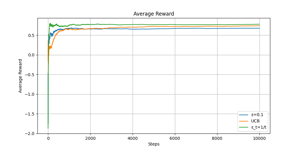
images/13-exploration/UCB_rewards.png
Upper confidence bound in comparison to ε-greedy with constant and scheduled ε.

Bayes’ theorem

Bayes’ theorem:

\[\begin{align*} p(A \cap B) &= p\agivenb{A}{B} p(B) \fragment{ = p\agivenb{B}{A} p(A) } \\ \Leftrightarrow \quad p\agivenb{B}{A} &= \frac{p\agivenb{A}{B} p(B)}{p(A)}. \end{align*}\]

\[\text{"Posterior"} = \frac{\text{"Likelihood"} \times \text{"Prior"}}{\text{"Evidence"}}.\]

  • Given new evidence \(A\),
  • we can update our prior estimate \(p(B)\)
  • to posterior estimate \(p\agivenb{B}{A}\)
  • using the likelihood of seeing the new evidence given \(B\).

Example: Medical testing

  • Imagine there is a rare disease that only \(1\%\) of the population has. There is a test for it which is \(90\%\) accurate.
  • You take the test and it comes back positive. What are the chances you actually have the disease?
  • Consider the two events \(A=\mathsf{sick}\) and \(B=\mathsf{positive~test}\): \[ p(A) = 0.01, \quad p\agivenb{B}{A}=0.9. \]
  • Total probability of the evidence (recall: \(p(A) + p(\neg A)=1\)): \[ p(B) = \underbrace{p\agivenb{B}{A}}_{\fragment{=0.9}} \underbrace{p(A)}_{\fragment{=0.01}} \fragment{ + \underbrace{p\agivenb{B}{\neg A}}_{\fragment{ =0.1 }} \underbrace{p(\neg A)}_{\fragment{=0.99}} } \fragment{ = 0.108. } \]
  • Posterior probability (prob. of having the disease given a positive test): \[p\agivenb{A}{B} = \frac{p\agivenb{B}{A} p(A)}{p(B)} \fragment{ = \frac{0.9 \cdot 0.01}{0.108} }\fragment{ = 0.0833 = 8.33\%. }\]

Thompson sampling

The idea behind Thompson sampling (also known as posterior sampling) is essentially Bayes’ theorem:

  • Start with a prior distribution over expected rewards (e.g., a Gaussian \(\Normal{\mu_{k}}{\sigma_{k}^2}\), \(k=1,\ldots,K\)).
  • Draw samples from the prior distribution to determine the next action.
  • Update to posterior distribution for the action that was selected and the reward that was observed.

Thompson sampling algorithm

For each step \(t = 1, 2, 3, \ldots\)

  1. Sample: For each arm \(k\), draw a random number \(\theta_k\) from its current posterior distribution: \(\theta_k \sim \Normal{\mu_{k}}{\sigma_k^2}\).
  2. Act: Select the arm with the highest sampled value: \(a_t = \arg\max(\theta_k)\).
  3. Observe: Pull that arm, receive reward \(r_t\).
  4. Update: Calculate the new \(\mu_k\) and \(\sigma_k^2\) for that specific arm.

Information gain and information-directed sampling

Information gain: “Which arm will give me the most valuable information to help me make better decisions in the future?”

Entropy and information gain

  • Let \(a^*\) be the true optimal action.
  • Goal: reduce uncertainty about \(a^*\).
  • Pulling \(a\) and observing \(r\): gain information.
  • Information gain (or mutual information) \(I\): expected entropy reduction of \(a^*\): \[I(a) = \Hc(a^*) - \ExpC{\Hc(a^*)}{r}.\]
    • \(I(a)\): How much pulling arm \(a\) will clarify which arm is truly the best.
    • If an arm’s reward distribution is highly uncertain, pulling yields a large information gain.
    • If we already know exactly what an arm does, pulling it yields zero information gain.

Information-directed sampling (IDS)

  • Maximizing information gain would waste our time testing highly unpredictable arms that we already know have poor rewards.
  • We need to consider the immediate loss, which we call regret (\(\Delta\)).
    • The expected regret of pulling arm \(a\) is the difference between the maximum possible expected reward and the expected reward of arm \(a\): \[\Delta(a) = \mathbb{E}[R(a^*)] - \mathbb{E}[R(a)]\]
    • Information-directed sampling (IDS) defines the information ratio for each arm: \[\Psi(a) = \frac{\Delta(a)^2}{I(a)}\]
    • “Cost-to-benefit” ratio: regret is the cost, information gain is the benefit.
    • A low ratio means we are either getting a high reward (low regret \(\Delta\)) or learning a lot about the system (high information gain \(I\)), or both.
  • IDS objective: \(a_t = \arg\min_{a\in\Ac}\Psi(a)\).

Summary

  • Optimistic exploration by estimating upper confidence bounds.
  • Posterior sampling: updating the belief of a reward (the prior) by using evidence \(\Rightarrow\) Bayes’ theorem.
  • Information gain: which actions give me the most information about the world?

Exploration in continuous spaces

Novelty-driven exploration: intrinsic motivation

  • As we have seen before (e.g., the UCB in Eq. \(\eqref{eq:Exp_UCB}\)), a common theme for exploration to add some form of bonus \(r^i\) to the reward signal that promotes exploration (also referred to as intrinsic reward, thus the superscript \(^i\)): \[ \hat{r} = r + r^i(N(s)). \]
  • This is a special case of the general concept of intrinsic motivation: We modify the reward signal in such a way that the agent is motivated (i.e., rewarded) to explore unknown territory: \[ \hat{r} = r + \beta r^i.\]
Type of intrinsic motivation Core question the agent asks Key algorithms
Novelty / information-theoretic “Have I seen this specific state configuration before?” Pseudo-counts (CTS, PixelCNN), count-based hashing
Prediction error / surprise “Can I predict what happens next if I take this action?” ICM (intrinsic curiosity module)
Knowledge gain / reduction of uncertainty “How much does this experience improve my model of the world?” RND (random network distillation), disagreement ensembles

The counting problem

  • As motivated in UCB (Eq. \(\eqref{eq:Exp_UCB}\)), we can add a bonus \(B\) to the reward that shrinks with the number of times we have seem certain state \(s\): \[ \begin{align*} \hat{r} &= r + r^i(N(s)) \\ \text{with}\quad s'&>s \Rightarrow N(s')< N(s). \end{align*} \]
  • But what does counting mean in continuous spaces?
images/13-exploration/Montezumas-Revenge.gif
Montezuma’s revenge.
  • Let’s revisit the Montezuma’s revenge example:
    • What if the key is placed slightly differently?
    • Or the spider?
    • Or some other minor detail?


The challenge in continuous \(\Sc\)

  • We “never” see the same thing twice (i.e., with probability zero).
  • However, some states are more similar than others.
    \(\Rightarrow\) back to function approximation.
Walker 2D (SAC).

Pseudo-counts

  • (Bellemare et al. 2016): Fit a density model \(p_\theta(s)\) (or \(p_\theta(s,a)\)).
  • \(p_\theta(s)\) may be high even for a new \(s\) if \(s\) is similar to previously seen states.
  • For small MDPs, the true (i.e., tabular) probability before and after a state visit is: \[\begin{align*} \text{Before:}\quad \underbrace{p(s)}_{\text{probability}\\ \text{/ density}} &= \underbrace{\overbrace{\frac{N(s)}{n}}}^{\text{count}}_{\text{total visits}} \\ \text{After:}\qquad p'(s) &= \frac{N(s)+1}{n+1}. \end{align*}\]
  • Can we use \(p_\theta(s)\) and \(p_{\theta'}(s)\) to get a pseudo-count \(\hat{N}(s)\)?
  • Bonus used by (Bellemare et al. 2016): \(r^i(\hat{N}(s)) = \sqrt{\frac{1}{\hat{N(s)}}}\).
  • Various alternatives available.

RL with pseudo-counts

  • Fit model \(p_\theta(s)\) to all states \(\Dc\) seen so far.
  • Take step \(t\) and osberve \(s_t\).
  • Fit new model \(p_{\theta'}(s)\) to \(\Dc \cup s_t\).
  • Set \(\hat{r}_t = r_t + r^i(\hat{N}(s))\).

Computing \(\hat{N}(s)\)

\[p_\theta(s_t) = \frac{\hat{N}(s_t)}{\hat{n}}, \qquad p_{\theta'}(s_t) = \frac{\hat{N}(s_t)+1}{\hat{n}+1}. \]

\(\Rightarrow\) Tow equations for two unknowns (\(\hat{N}\) and \(\hat{n}\))!

\[\begin{align*} \hat{N}(s_t) &= \hat{n} p_\theta(s_t), \qquad \hat{n} = \frac{1-p_{\theta'}(s_t)}{p_{\theta'}(s_t)-p_{\theta}(s_t)},\\ \hat{N}(s_t) &= \frac{\cbracket{1-p_{\theta'}(s_t)}p_\theta(s_t)}{p_{\theta'}(s_t)-p_{\theta}(s_t)} . \end{align*} \]

Example: Count-based exploration in Atari games

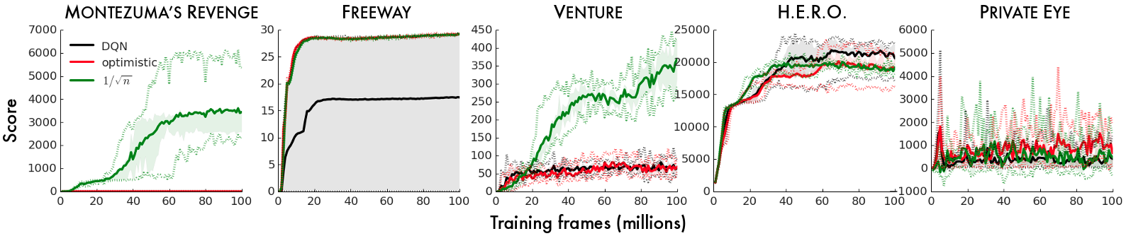
images/13-exploration/count-based-results-montezuma.png
Exploration of rooms/levels in Montezuma’s revenge (Bellemare et al. 2016).


images/13-exploration/count-based-results.png
Performance on various Atari games (Bellemare et al. 2016).

Ways to estimate the density

  • There are numerous ways to estimate the state density \(p_\theta(s)\) or state-action density \(p_\theta(s,a)\).
  • Key takeaways:
    • \(p_\theta(s)\) does not need to produce great samples \(s\).
    • It just needs to yield a good approximation of the state density distribution!

Curiosity-driven exploration

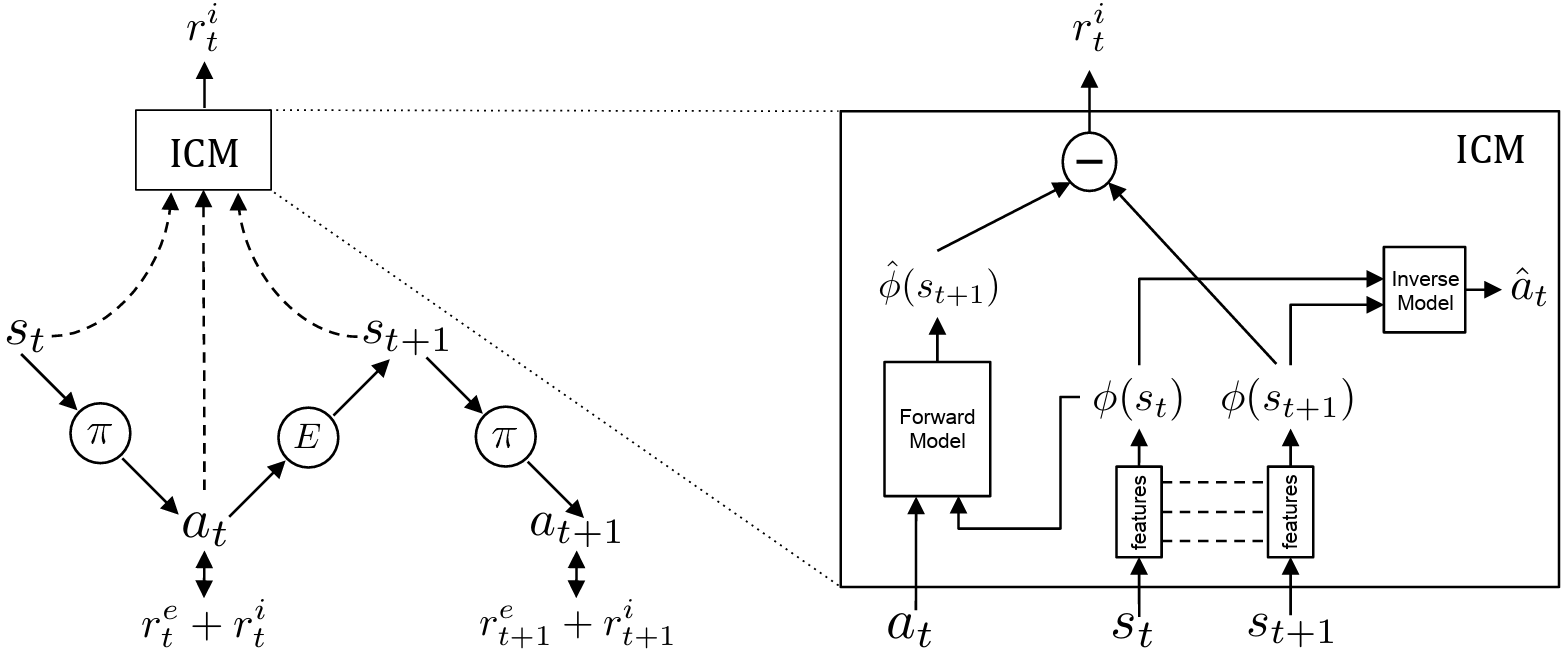
Instead of counting states, an Intrinsic Curiosity Module (ICM) (Pathak et al. 2017) uses a predictive neural network model:

  • The agent in state \(s_t\) executes \(a\sim\pi\) \(\Longrightarrow\) \(s_{t+1}\).
  • \(\pi\) is trained to maximize the sum of the extrinsic reward (\(r^e_t\)) by the environment \(E\) and the intrinsic reward (\(r^i_t\)) generated by the ICM: \[r_t = r_t^e + r_t^i.\]
  • ICM: The prediction error in feature space is used as the curiosity based intrinsic reward signal \(r^i_t\).
    • The forward model takes as inputs \(\phi(s_t)\) and \(a_t\) and predicts the feature representation \(\hat\phi(s_{t+1})\) of \(s_{t+1}\).
    • ICM encodes \(s_t\), \(s_{t+1}\) into the features \(\phi(s_t)\), \(\phi(s_{t+1})\) that are trained to predict \(a_t\) (the inverse dynamics model).
images/13-exploration/ICM.png
Intrinsic Curiosity Module (Pathak et al. 2017).
  • “The inverse model helps learn a feature space that encodes information relevant for predicting the agent’s actions only and the forward model makes this learned feature representation more predictable.” (Pathak et al. 2017)
    • The inverse model only keeps track of things in the environment that the agent’s actions can actually influence.
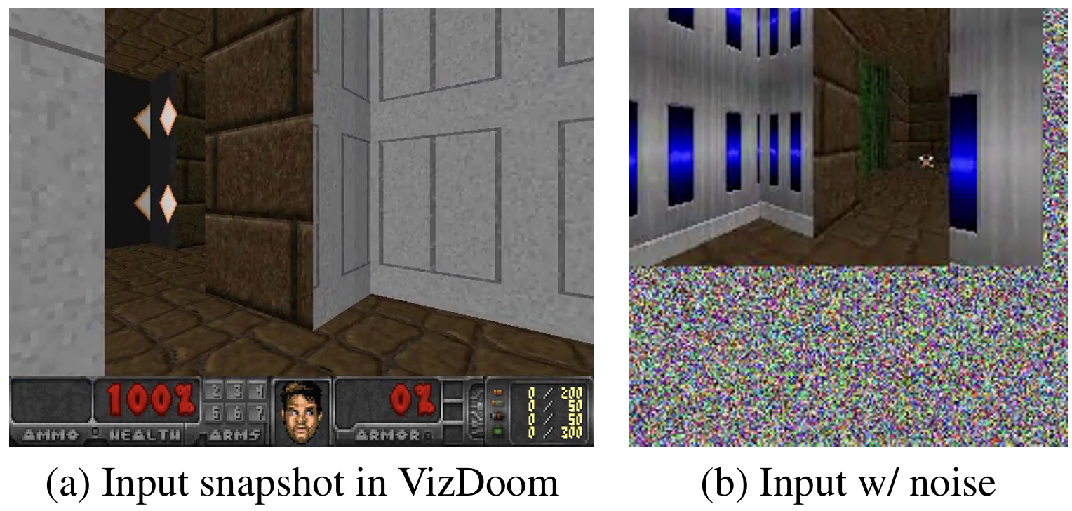
    • If a TV screen shows random noise, the network filters it out because the agent’s actions didn’t cause it. The agent won’t feel “curious” about it.

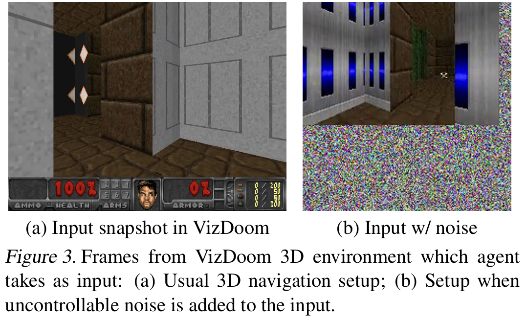
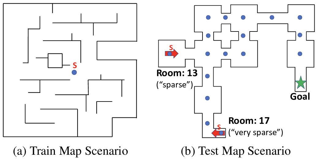
Example: VizDoom 3D “My way home” (1)

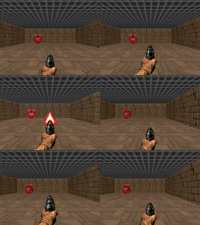
  • Inspired by the classic video game “Doom”, avialable via Gymnasium.
  • Task: Reach a goal
    \(\Rightarrow\) very sparse reward.
  • Pre-training using curiosity only!
images/13-exploration/VizDoomBasic-Doom2.gif
Basic scenario
images/13-exploration/VizDoomMyWayHome-Screenshots.png
Source: (Pathak et al. 2017).
images/13-exploration/VizDoomMyWayHome-Maps.png
Source: (Pathak et al. 2017).
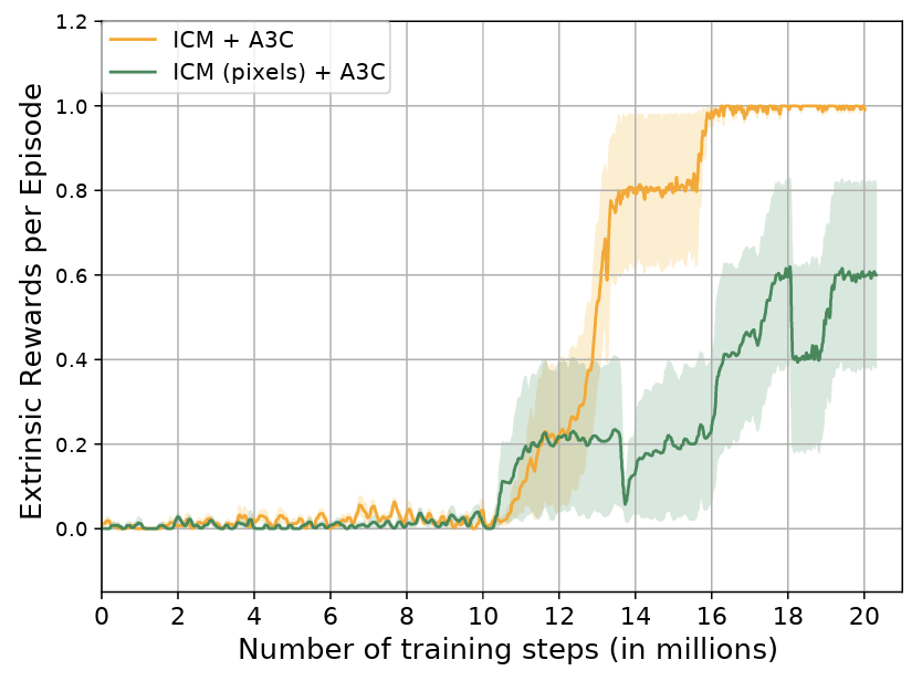
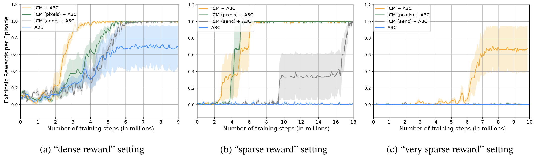
  • Comparison using the A3C algorithm (Mnih et al. 2016): This is an extension of policy gradients with improved, asynchronous replay buffer and an actor for continuous actions (by now largely replaced by PPO).
    • A3C: the standard algorithm with \(\epsilon\)-greedy exploration
    • ICM + A3C: the ICM-enhanced version ()
    • two variants of (ICM + A3C) with some functionalities turned off (so-called ablations to assess the value of these parts)
      • ICM (pixels) + A3C: direct assessment of the pixels; no use of the backward model to identify the action-relevant pieces of the input.
      • ICM (aenc) + A3C: curiosity is computed using the features of pixel-based forward model.

Example: VizDoom 3D “My way home” (2)

images/13-exploration/VizDoomMyWayHome-Exploration.pngExploration: ICM (green) versus random exploration (blue).
images/13-exploration/VizDoomMyWayHome-Rewards.png
images/13-exploration/VizDoomMyWayHome-Screenshots2.png
images/13-exploration/VizDoomMyWayHome-RewardsNoise.png
Robustness with 40 % noisy pixels.

Novelty vs. Curiosity

Feature Novelty methods (e.g., count-based) Intrinsic curiosity (e.g., ICM)
Core question “Have I stood in this exact spot before?” “Can I accurately predict what will happen if I push this button?”
Mechanism Tracks visitation counts or state densities. Measures the prediction error of a forward-dynamics neural network.
The “TV Screen” vulnerability Vulnerable. A TV screen cycling random images represents infinite novel states. Handled via feature encoding. It ignores randomness it cannot control.
Best suited for Environments with static, clean states where visiting everything matters (e.g., Montezuma’s Revenge). Dynamic environments with visual noise where learning the “physics” of the world is required.

Exploration via posterior sampling in DRL

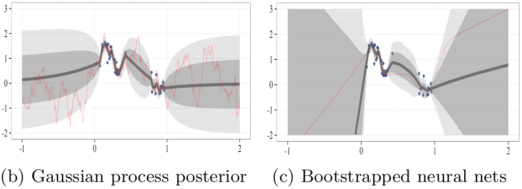
Bootstrapped DQN (Osband et al. 2016)

  • Instead of training a single neural network, we train an ensemble of \(K\) networks (typically \(K=10\)).
  • We use standard boostrapping from supervised learning and random masking of individual samples to diversify between the different models.
  • During each episode, we randomly select one model and then follow this model to the end.
  • How this solves the exploration-exploitation dilemma:
    • Disagreement between different models
      \(\Rightarrow\) High uncertainty
      \(\Rightarrow\) Exploration over various runs.
    • Agreement between different models
      \(\Rightarrow\) Low uncertainty
      \(\Rightarrow\) Exploitaiton of known good behavior.

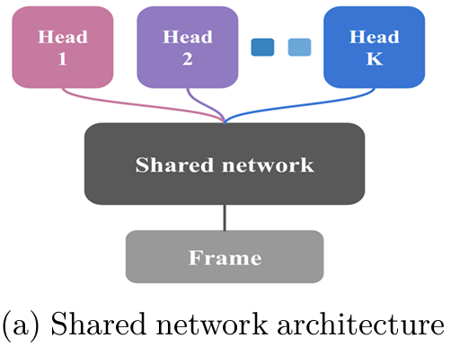
The challenge: training multiple networks!

Approach: Single network with \(K\) heads!
images/13-exploration/bootstrappedDQN-1.png
images/13-exploration/bootstrappedDQN-2.png

Random network distillation

RND (Burda et al. 2019) uses two neural networks that consider the same state \(s\), but they have different jobs:

  1. The target network \(f(s)\) is a neural network that is initialized randomly and then never changed.
    Think of it as a some oracle that takes the state (e.g., the pixels of the screen) and outputs a random string of numbers.
  2. The predictor network \(f_\theta(s)\) is allowed to learn. Its job is to guess what the target network’s output will be.

\[\Rightarrow\text{ Intrinsic reward:} \quad r^i = \norm{f_\theta(s) - f(s)}^2.\]

How does this create “curiosity”?

  • Familiar territory: we see similar states \(s\) multiple times \(\Rightarrow\) We can learn what \(f(s)\) predicts \(\Rightarrow\) The prediction error is small.
  • Unexplored territory: In states that the predictor has not seen, it has to “guess” at the target \(\Rightarrow\) The prediction error is large.

RND solves the “Noisy TV problem”

  • Other curiosity methods reward the agent if it cannot predict the next frame of the game.
  • If we encounter a noisy TV, the agent remains curious for ever, as it cannot predict the outcome.
  • RND fixes this:
    • If the agent sees a TV with static, the target \(f(s)\) gives a constant, predictable output for that specific pattern.
    • The predictor network \(f_\theta(s)\) can quickly learn that pattern.
    • The error drops to zero, and the agent moves on to explore truly novel states.
[Source: OpenAI blog]

RND versus next-state-prediction

leaderboard29 leaderboard29 [Source: OpenAI blog]

  • Instead of predicting some meaningful next state, matching random features simplifies the learning process.
  • Learning a model may still be very helpful, though, when we use it for additional tasks (e.g., model-based RL).

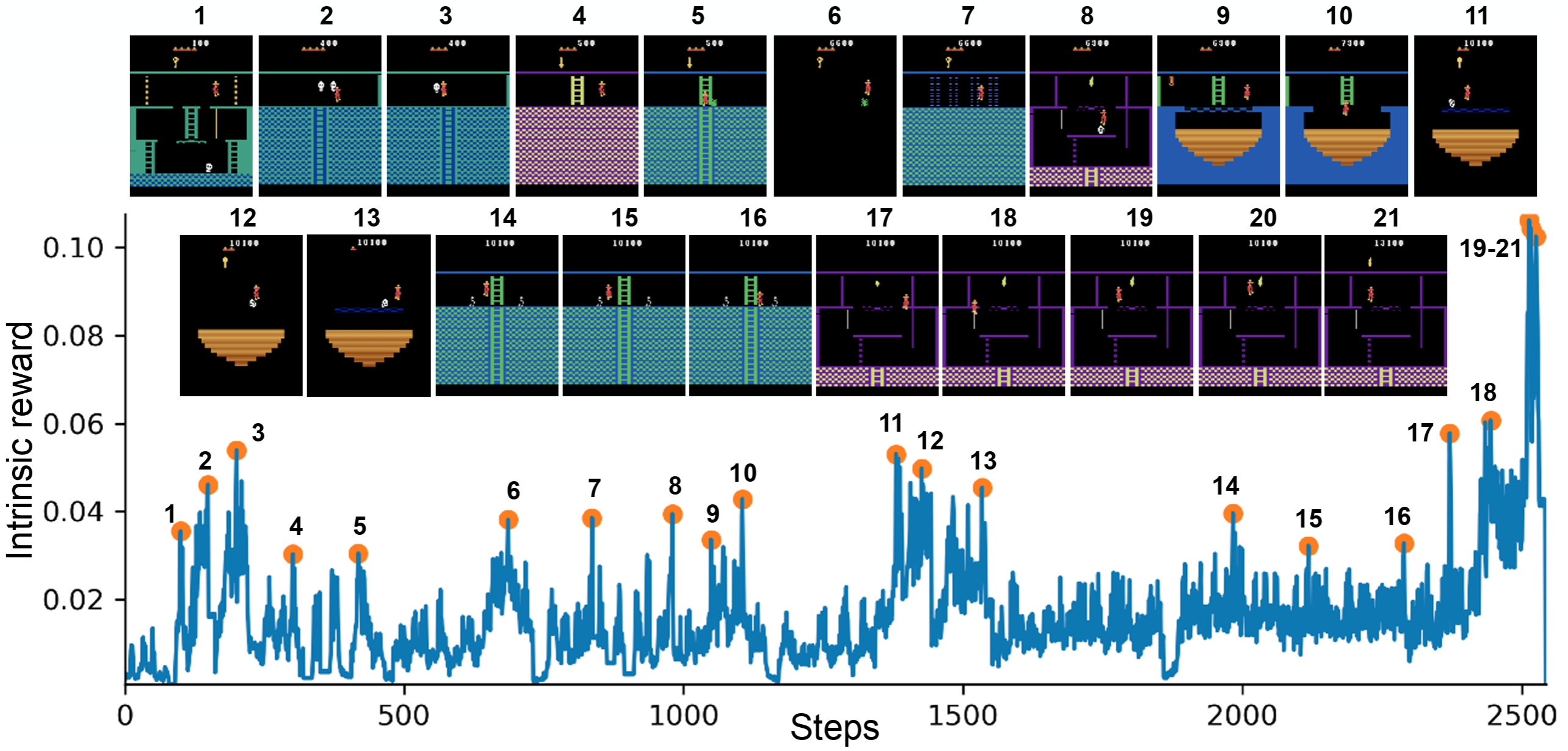
Example: Montezuma’s revenge

Discovery of new rooms to satisfy curiosity. Then revisiting those rooms to maximize the extrinsic reward. [Source: OpenAI blog]
images/13-exploration/RND-montezuma.png
Spikes in the intrinsic reward at new events (Burda et al. 2019).


Good performance also for Super Mario. [Source: OpenAI blog]

Comparison between ICM and RND

Feature Intrinsic Curiosity Module (ICM) Random Network Distillation (RND)
Core Mechanism Predicts the next state given the current state and action (forward dynamics). Predicts the output of a fixed, randomly initialized neural network on the current state.
The “Noisy TV” problem Vulnerable. If a screen shows unpredictable random noise, ICM gets trapped staring at it because prediction error remains high. Immune. The random target network outputs a completely deterministic (though random) function. The predictor network learns it quite easily, dropping the reward to zero.
Complexity High. Requires training three sub-networks: an encoder, an inverse dynamics model, and a forward dynamics model. Low. Requires training only one network (the predictor) to match a frozen, untrained target network.
Scalability Harder to scale because compounding forward-prediction errors in high-dimensional state spaces create erratic reward signals. Highly scalable. It handles raw very exceptionally well (and famously allowed PPO to crack Montezuma’s Revenge).

Relation between exploration and reward shaping

The fundamental difference between exploration and reward shaping lies in who defines the reward and why.

  • Reward Shaping: top-down approach where a human engineer hard-codes external hints into the environment.
  • Model Curiosity: bottom-up approach where the agent generates its own internal rewards based on surprise and ignorance.

Reward shaping (the human guide)

  • Instead of only giving the agent a sparse reward at the end of an episode, we add a function that rewards the agent for reaching partial objectives.
  • For example, every step that reduces the straight-line distance to the goal might give the agent a small bonus.

Drawback: unintended side effects

  • Reward shaping can quickly cause unintended side effects if not done perfectly.
  • Since humans are essentially telling the agent how to solve the problem rather than just what the problem is, the agent will often find loopholes to maximize the shaped reward without solving the actual task.
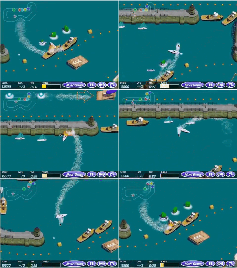
  • Popular Example: Boat-racing video game.
    • Researchers shaped the reward by giving the boat points for hitting targets along the track.
    • Instead of finishing the race, the agent learned to drive in circles, infinitely loops through a specific cluster of targets, and constantly set itself on fire because doing so yielded more points than winning the actual race.
images/13-exploration/boat-racing.gif

Summary / what we have learned today

  • Various ways to encourage seeing previously unknown territory.
    • Pseudo-counts to “count” how often states have been seen, then benefit unknown states.
    • Bayes’ theorem / Thompson sampling to update the belief of a reward.
    • Information gain to select states that we believe to yield a lot of new information.
  • Intrinsic curiosity can be realized by adding rewards for previously unseen situations.
    • Novelty vs. curiosity: “Which states haven’t been seen yet?” vs. “Let’s go where we cannot predict what’s going to happen.”
  • Bootstrapping over ensembles of DQNs can also allow us to identify hard-to-predict territory (disagreement in the ensemble).

References

Bellemare, Marc, Sriram Srinivasan, Georg Ostrovski, Tom Schaul, David Saxton, and Remi Munos. 2016. “Unifying Count-Based Exploration and Intrinsic Motivation.” In Advances in Neural Information Processing Systems, edited by D. Lee, M. Sugiyama, U. Luxburg, I. Guyon, and R. Garnett. Vol. 29. Curran Associates, Inc.
Burda, Yuri, Harrison Edwards, Amos Storkey, and Oleg Klimov. 2019. “Exploration by Random Network Distillation.” In International Conference on Learning Representations. https://openreview.net/forum?id=H1lJJnR5Ym.
Ferreira, Rafael Pereira, Emil Schubert, and Américo Scotti. 2024. “Exploring Multi-Armed Bandit (MAB) as an AI Tool for Optimising GMA-WAAM Path Planning.” Journal of Manufacturing and Materials Processing 8 (3).
Fu, Justin, John Co-Reyes, and Sergey Levine. 2017. “EX2: Exploration with Exemplar Models for Deep Reinforcement Learning.” In Advances in Neural Information Processing Systems, edited by I. Guyon, U. Von Luxburg, S. Bengio, H. Wallach, R. Fergus, S. Vishwanathan, and R. Garnett. Vol. 30. Curran Associates, Inc. https://proceedings.neurips.cc/paper_files/paper/2017/file/1baff70e2669e8376347efd3a874a341-Paper.pdf.
Haarnoja, Tuomas, Aurick Zhou, Kristian Hartikainen, George Tucker, Sehoon Ha, Jie Tan, Vikash Kumar, et al. 2018. “Soft Actor-Critic Algorithms and Applications.” arXiv:1812.05905.
Mnih, Volodymyr, Adria Puigdomenech Badia, Mehdi Mirza, Alex Graves, Timothy Lillicrap, Tim Harley, David Silver, and Koray Kavukcuoglu. 2016. “Asynchronous Methods for Deep Reinforcement Learning.” In Proceedings of the 33rd International Conference on Machine Learning, edited by Maria Florina Balcan and Kilian Q. Weinberger, 48:1928–37. Proceedings of Machine Learning Research. New York, New York, USA: PMLR. https://proceedings.mlr.press/v48/mniha16.html.
Osband, Ian, Charles Blundell, Alexander Pritzel, and Benjamin Van Roy. 2016. “Deep Exploration via Bootstrapped DQN.” In Advances in Neural Information Processing Systems, edited by D. Lee, M. Sugiyama, U. Luxburg, I. Guyon, and R. Garnett. Vol. 29. Curran Associates, Inc. https://proceedings.neurips.cc/paper_files/paper/2016/file/8d8818c8e140c64c743113f563cf750f-Paper.pdf.
Ostrovski, Georg, Marc G. Bellemare, Aäron van den Oord, and Rémi Munos. 2017. “Count-Based Exploration with Neural Density Models.” In Proceedings of the 34th International Conference on Machine Learning, edited by Doina Precup and Yee Whye Teh, 70:2721–30. Proceedings of Machine Learning Research. PMLR. https://proceedings.mlr.press/v70/ostrovski17a.html.
Pathak, Deepak, Pulkit Agrawal, Alexei A. Efros, and Trevor Darrell. 2017. “Curiosity-Driven Exploration by Self-Supervised Prediction.” In Proceedings of the 34th International Conference on Machine Learning, edited by Doina Precup and Yee Whye Teh, 70:2778–87. Proceedings of Machine Learning Research. PMLR. https://proceedings.mlr.press/v70/pathak17a.html.
Tang, Haoran, Rein Houthooft, Davis Foote, Adam Stooke, OpenAI Xi Chen, Yan Duan, John Schulman, Filip DeTurck, and Pieter Abbeel. 2017. “#Exploration: A Study of Count-Based Exploration for Deep Reinforcement Learning.” In Advances in Neural Information Processing Systems, edited by I. Guyon, U. Von Luxburg, S. Bengio, H. Wallach, R. Fergus, S. Vishwanathan, and R. Garnett. Vol. 30. Curran Associates, Inc. https://proceedings.neurips.cc/paper_files/paper/2017/file/3a20f62a0af1aa152670bab3c602feed-Paper.pdf.