Deep Reinforcement Learning

Optimal Control & Feedback Control

Prof. Dr. Sebastian Peitz

Chair of Safe Autonomous Systems, TU Dortmund

Summer term 2026

🚀 by Decker

Content

Recap of model-free RL
Open-loop optimal control
- Trajectory planning
- Solution approaches
- Stochastic optimal control
- The linear case
Closed-loop control
- Model Predictive Control (MPC)
- Differentiable Predictive Control (DPC)

Where are we?

Lecture contents
Chapter	Topic	Content
	Basics & tabular methods
1-5	Bandits, MDPs, Dynamic Programming, Monte Carlo, TD Learning	RL basics in finite dimensions
	Deep-learning-based methods
6-13	DQN, policy gradients, actor-critic, PPO/SAC, exploration	Deep RL from basics to modern algorithms
	Model-Based Control
14	Optimal control & feedback control	How to do control when we know the model
	Model-based reinforcement learning
	Advanced Topics

Recap: model-based and model-free RL

Until now, knowledge of a model only in the simplest RL approaches.
- Dynamic Programming for tabular RL, e.g., policy or value iteration.
- We need to know $\textcolor{red}{\psprimesa}$ to update our value estimate!
All the advanced algorithms: model-free RL.
- Collect experience by following the current policy $\pi$,
- then update our estimate of $V$, $Q$, $A$ or $\pi$ only from the data.

Algorithm: Value iteration for estimating $\pi\approx \pi^*$.

while ($\Delta > \theta$):
$\quad$ $\Delta \gets 0$
$\quad$ for $s \in \Sc$:
$\quad\quad$ $V_{\mathsf{old}}(s) \gets V(s)$
$\quad\quad$ $V(s) \gets \max_{a\in\Ac} \sum_{s'\in\Sc} \textcolor{red}{\psprimesa} \left[ r + \gamma V(s') \right]$
$\quad\quad$ $\Delta \gets \max(\Delta, \abs{V_{\mathsf{old}}(s)-V(s)})$

Advantages / disadvantages of model-free RL

$\textcolor{green}{\mathbf{+}\text{ No model knowledge required. All we need is access\\ ~~~~to the system / a black-box simulator.}}$
$\textcolor{green}{\mathbf{+}\text{ No bias due to inaccurate model.}}$

$\textcolor{green}{\mathbf{+}\text{ Easier to implement.}}$
$\textcolor{red}{\mathbf{-}\text{ Data-hungry! Can be very sample-inefficient.}}$ $\textcolor{red}{\mathbf{-}\text{ Ignorant of prior knowledge.}}$

Today: Can we do better if we know the dynamics?

We often know the dynamics:

Games (e.g., Chess, Go, Atari games).
Easily modeled systems (e.g., car navigation).
Simulated environments (e.g., robotics, video games)

Also, we can often learn the dynamics:

System identification: fit unknown parameters of a known model.
Learning: fit a general purpose model to observed transition data.

What is a model?

Very generally, a model is an MDP tuple $(\Sc, \Ac, p, r, \gamma)$, just as we have seen before. Most notably, we have
- the dynamics model $\psprimesa$,
- the reward probability $r \sim \pC{\cdot}{s,a}$.
The state and action spaces $\Sc$ and $\Ac$ are usually assumed to be known.
The discount factor is given or can be chosen by an expert.

Types of models

1. Probabilistic vs. deterministic

probabilistic: \[s' \sim \pC{\cdot}{s,a},\quad r \sim \pC{\cdot}{s,a}.\]
deterministic (a special case of the former): \[s' = f(s,a), \quad r=\ell(s,a).\]

2. Known vs. unknown

True MDP: $p$ and $r$ (or $f$ and $\ell$) are perfectly known a priori.
Approximated MDP: $p$ and $r$ (or $f$ and $\ell$) need to be learned, \[p_\theta \approx p,~ r_\phi \approx r \qquad \text{or} \qquad f_\theta\approx f,~ \ell_\phi \approx \ell. \]

Open-loop optimal control

Planning & optimal control

For now, we asumme that the model
- is known,
- is fully deterministic.
In the episodic case ($T<\infty$), the RL problem becomes \[\begin{equation}\begin{aligned} &\min_{a_0,\ldots,a_{T-1}} \sum_{t=0}^T \ell(s_t,a_t) = \min_{a_0,\ldots,a_{T-1}} L(a) \\ \text{subject to}\quad &s_{t+1}=f(s_t,a_t),~t=0,1,\ldots,T-1. \end{aligned}\label{eq:OC_ocp} \end{equation} \]
Eq. $\eqref{eq:OC_ocp}$ is referred to as an optimal control problem (OCP).
- $\ell$ is the stage cost.
  💡 Closely related to the negative reward $-r$!
- $L$ is the cost that we seek to minimize.
  💡 Closely related to value $V$!
- Optimal control is usually formulated as a minimization problem, e.g., the distance to a desired trajectory.
Generally, optimal control refers to the open-loop / planning setting.

Inspired by Sergey Levine’s CS285 lecture.

The deterministic vs. the stochastic case

In RL, we usually assume that we have a stochastic problem for various reasons:
- stochastic dynamics,
- stochastic actions/policies,
- stochastic rewards.
In the open-loop setting, stochastic optimal control is suboptimal!
$\Rightarrow$ Why?

Stochastic dynamics

\[ \pC{s_0,\ldots,s_T}{a_0,\ldots,a_{T-1}} = p(s_0)\prod_{t=0}^{T-1}\pC{s_{t+1}}{s_t,a_t}.\]

The optimal action $a_1$ depends on $s_1$, which we cannot know for certain at $t=0$.
The same is true for all following states and actions.

Some approaches for stochastic optimal control

Certainty Equivalence (CE)
- Simply replace all stochastic quantities by their expectations/mean values.
  $\textcolor{green}{\mathbf{+}\text{ Computationally cheap.}}$
  $\textcolor{red}{\mathbf{-}\text{ Completely ignores variance.}}$
Mean-variance / risk-sensitive optimization
- define loss function composed of mean and variance: \[\min_a \Exp{L} + \gamma\, \Var{L}.\] $\textcolor{green}{\mathbf{+}\text{ Accounts for variance.}}$
  $\textcolor{red}{\mathbf{-}\text{ Need additional compute to estimate $\Var{L}$.}}$
Sample-path optimization
- Monte-Carlo estimate of expected loss by multiple simulations with different noise realizations $\omega_i$: \[ \min_a \frac{1}{N} \sum_{i=1}^N L(a,\omega_i).\] $\textcolor{green}{\mathbf{+}\text{ Can estimate arbitrary distributions (beyond Guassian).}}$
  $\textcolor{red}{\mathbf{-}\text{ Compute grows with }N.}$

Solving the OCP: single shooting

\[\begin{equation}\begin{aligned} &\min_{a_0,\ldots,a_{T-1}} \underbrace{\sum_{t=0}^T \ell(s_t,a_t)}_{= L(a)} \quad \text{subject to}\quad &s_{t+1}=f(s_t,a_t),~t=0,1,\ldots,T-1. \end{aligned}\tag{\ref{eq:OC_ocp}} \end{equation} \]

A very common approach to solve the OCP $\eqref{eq:OC_ocp}$ is via single shooting, where assume that the states $s_t$ are implicitly defined by choosing the actions $a_t$.
💡 This holds for most systems of interest. The basis for this are existence-and-uniqueness theorems, e.g., by Picard-Lindelöf.

Single shooting

Initialize: Initial state $s_0$, action sequence $\iterate{a}{0}=\cbracket{\iteratesub{a}{0}{0},\ldots,\iteratesub{a}{0}{T-1}}$.

for $j=0,1,2,\ldots$:
$\quad$ simulate the system following $\iterate{a}{j}$ to get $\iterate{s}{j}=\cbracket{\iteratesub{s}{j}{1},\ldots,\iteratesub{s}{j}{T}}$
$\quad$ assess the performance by computing $L\cbracket{\iterate{a}{j}}$
$\quad$ gradient descent to update our actions: \[\iterate{a}{j+1} = \iterate{a}{j} - \eta \nabla_a L\cbracket{\iterate{a}{j}} \]

Remaining question:

How do we compute the gradient \[\nabla_a L\cbracket{\iterate{a}{j}}?\]

Gradients in single shooting (1)

The procedure of computing the gradient is closely related to the backpropagation algorithm!

Turn the constraint into an objective via the Lagrangian formalism, where $\lambda$ is the adjoint state: \[\begin{align*} \Lc(s,a,\lambda) = &\sum_{t=0}^T \ell(s_t,a_t) + \sum_{t=0}^{T-1} \lambda^\top_{t+1}\cbracket{f(s_t,a_t)- s_{t+1}} \\ =&\rbracket{\ell(s_0,a_0) + \lambda^\top_{1}f(s_0,a_0)} + \rbracket{\ell(s_1,a_1) + \lambda^\top_{2}f(s_1,a_1) -\lambda^\top_{1} s_1} + \ldots + \\ &\rbracket{\ell(s_t,a_t) + \lambda^\top_{t+1}f(s_t,a_t) -\lambda^\top_{t} s_{t}} + \ldots + \rbracket{\ell(s_T,a_T) + \lambda^\top_{T} s_T}. \end{align*}\]
Necessary condition for optimality: Total derivative of $\Lc$ has to be zero: \[ \pdiff{\Lc}{\lambda_t} = 0,\quad \pdiff{\Lc}{s_t} = 0, \quad \pdiff{\Lc}{a_t} = 0. \]

Gradients in single shooting (2)

\[\Lc(s,a,\lambda) = \sum_{t=0}^T \ell(s_t,a_t) + \sum_{t=0}^{T-1} \lambda^\top_{t+1}\cbracket{f(s_t,a_t)- s_{t+1}}\]

State equation: \[\pdiff{\Lc}{\lambda_t} = s_{t} - f(s_{t-1},a_{t-1}) \stackrel{!}{=} 0 \fragment{ \quad \Leftrightarrow \quad s_{t+1} = f(s_t,a_t) \quad \text{for }t=0,\ldots,T-1. }\]
Adjoint equation: \[\pdiff{\Lc}{s_t} = \pdiff{\ell}{s_t} + \cbracket{\pdiff{f}{s_t}}^\top\lambda_{t+1} - \lambda_t \stackrel{!}{=} 0 \fragment{ \quad \Leftrightarrow \quad \lambda_{t} = \pdiff{\ell}{s_t} + \cbracket{\pdiff{f}{s_t}}^\top\lambda_{t+1} \quad \text{for }t=0,\ldots,T-1. }\]
Final adjoint state ($t=T$): No influence on a future state, $\lambda_T = \pdiff{\ell}{s_T}$.
Action gradient: \[\pdiff{\Lc}{a_t} = \pdiff{\ell}{a_t} + \cbracket{\pdiff{f}{a_t}}^\top\lambda_{t+1} \quad \text{for }t=0,\ldots,T-1. \]

Gradients in single shooting (3)

Gradient calculation in the single shooting method for solving $\eqref{eq:OC_ocp}$

Given: Initial state $s_0$, action sequence $a=\cbracket{a_0,\ldots,a_{T-1}}$.

Forward simulation of the state equation: \[s_{t+1} = f(s_t,a_t), \qquad t=0,1,\ldots,T-1.\]
“Initial condition” (i.e., at final time $T$) for the adjoint equation: $\lambda_T = \pdiff{\ell}{s_T}.$
Backward simulation of the adjoint equation: \[\lambda_{t} = \pdiff{\ell}{s_t} + \cbracket{\pdiff{f}{s_t}}^\top\lambda_{t+1}, \qquad t=T-1,T-2,\ldots,1,0.\]
Gradient calculation w.r.t. $a$: \[\pdiff{\Lc}{a_t} = \pdiff{\ell}{a_t} + \cbracket{\pdiff{f}{a_t}}^\top\lambda_{t+1}, \qquad t=0,1,\ldots,T-1.\]

Notes

The backward simulation is closely related to the backward pass in backpropagation.
In modern packages such as PyTorch, JAX or TensorFlow, this procedure can be automated with autodiff, when appropriately implementing the forward pass.

Solving the OCP: full discretization

Alternative to forward-backward: the full discretization
Both $s$ and $a$ become optimization variables: \[ x=\rbracket{s_0^\top, a_0^\top,s_1^\top,a_1^\top,\ldots, a_{T-1}^\top,s_T^\top}^\top. \]
Reformulation of the OCP $\eqref{eq:OC_ocp}$ \[\begin{equation} \min_{x} F(x) = \sum_{t=0}^T \ell(s_t,a_t) \quad\text{s.t.}\quad C(x) = \begin{bmatrix} f(s_0,a_0) - s_1 \\ f(s_1,a_1) - s_2 \\ \vdots \\ f(s_{T-1},a_{T-1}) - s_T \end{bmatrix}=0 \label{eq:OC_ocp_discretized} \end{equation} \]
Total number of optimization variables when the state dimension is $n$ and the action dimension is $m$: $(T+1)n + Tm$.
Solution via standard solvers for nonlinear, constrained optimization problems:
- Requires the gradients $\nabla_x F(x)$ and $\nabla_x C(x)$.
- The latter is a very large matrix, but it is fortunately very sparse.

Comparison: Shooting vs. full discretization

	Shooting $\eqref{eq:OC_ocp}$	Full discretization $\eqref{eq:OC_ocp_discretized}$
Sensitivity to initialization	Very sensitive to poor initial guesses $\iterate{a}{0}$.	Because we initialize the entire state trajectory $s$, the system doesn’t have to be dynamically feasible during early solver iterations $\Rightarrow$ Significantly more stable for unstable dynamics.
Computational cost vs. convergence	Fast iterations (one forward and backward pass), but may take many iterations to converge.	Iterations more expensive, but standard Sequential Quadratic Programming (SQP) or Interior Point methods achieve quadratic convergence near the solution, requiring far fewer total iterations.
Constraint Handling	Handling state constraints requires challenging penalty functions or barrier methods.	Limits on states like $s_{\mathsf{min}} \leq s_t \leq s_{\mathsf{max}}$ or actuations ($a_{\mathsf{min}} \leq a_t \leq a_{\mathsf{max}}$) can be handled easily. They are simply treated as bound constraints on elements of our vector $x$.

The linear-quadratic case

Let’s consider a special (yet very common) case

Linear dynamics: \[s_{t+1}=A s_t + B a_t, \quad\text{with }A\in\R^{n\times n}\text{ and }B\in\R^{n \times m}.\]
Quadratic losses: \[L(s,a) = \cbracket{\sum_{t=0}^{T-1} s_t^\top Q s_t + a_t^\top R a_t} + s_T^\top Q_f s_T,\] with matrices $Q,Q_f\in\R^{n\times n}$ penalizing the (terminal) state and
$R\in\R^{m\times m}$ penalizing the control cost.

Additional conditions

The matrix $Q$ is positive semidefinite: \[s^\top Q s \geq 0 ~\forall~s\in\R^n.\]
The matrix $R$ is positive definite: \[a^\top R a > 0 ~\forall~a\in\R^m.\]
These ensure existence and uniquenes of a minimizer $s^*,a^*$.

Linear-quadratic optimal control problem

\[\begin{equation} \begin{aligned} \min_{s,a} &\cbracket{\sum_{t=0}^{T-1} s_t^\top Q s_t + a_t^\top R a_t} + s_T^\top Q_f s_T \\ \text{subject to}\quad s_{t+1}&=A s_t + B a_t,~t=0,1,\ldots,T-1. \end{aligned} \label{eq:OC_ocp_linear} \end{equation}\]

Removing the constraints

Let’s explicitly calculate $s_1,s_2,\ldots$: \[\begin{align*} &s_1 = \textcolor{blue}{A s_0 + B a_0} \\ &s_2 = A s_1 + B a_1 \fragment{ = A (\textcolor{blue}{A s_0 + B a_0}) + B a_1 } \fragment{ = \textcolor{red}{A^2 s_0 + AB a_0 + B a_1} } \\ &s_3 = A s_2 + B a_2 \fragment{ = A (\textcolor{red}{A^2 s_0 + AB a_0 + B a_1}) + B a_2 }\fragment{ = A^3 s_0 + A^2B a_0 + ABa_1 + Ba_2 } \\ &\text{General rule:} \quad s_t = A^t s_0 + \sum_{i=0}^t A^{t-i-1}B a_i\\ &\text{Explicitly:} \quad \underbrace{\begin{bmatrix} s_0 \\ s_1 \\ s_2 \\ s_3 \\ \vdots \\ s_T \end{bmatrix}}_{\hat{s}\in\R^{(T+1)n}} = \underbrace{\begin{bmatrix} 0 & 0 & 0 & \ldots & B \\ 0 & 0 & 0 & \ldots & 0 \\ AB & B & 0 & \ldots & 0 \\ A^2B & AB & B & \ddots & 0 \\ \vdots & \vdots & \vdots & \ddots & \vdots \\ A^{T-1}B & A^{T-2}B & A^{T-3}B & \ldots & B \\ \end{bmatrix}}_{G\in\R^{(T+1)n\times Tm}} \underbrace{\begin{bmatrix} a_0 \\ a_1 \\ a_2 \\ a_3 \\ \vdots \\ a_{T-1} \end{bmatrix}}_{\hat{a}\in\R^{Tm}} + \underbrace{\begin{bmatrix} I \\ A \\ A^2 \\ A^3 \\ \vdots \\ A^T \end{bmatrix}}_{H\in\R^{(T+1)n}} s_0 \\ &\text{In short:}\quad \hat{s}=G\hat{a}+Hs_0 \end{align*}\]

Reformulating the cost function

Next, we stack our penalty matrices such that they match the dimensions of $S$ and $U$: \[ \hat{Q} = \begin{bmatrix} Q & & & \\ & \ddots & & \\ & & Q & \\ & & & Q_f \end{bmatrix}\in\R^{(T+1)n \times (T+1)n}, \qquad \hat{R} = \begin{bmatrix} R & & \\ & \ddots & \\ & & R \end{bmatrix}\in\R^{Τm\times Tm}. \]
We can now insert this into the linear-quadratic OCP $\eqref{eq:OC_ocp_linear}$: \[\begin{align*} \min_{s,a} \cbracket{\sum_{t=0}^{T-1} s_t^\top Q s_t + a_t^\top R a_t} + s_T^\top Q_f s_T \quad &\text{s.t.}\quad s_{t+1}=A s_t + B a_t,~t=0,1,\ldots,T-1 \\ \text{becomes}\qquad\qquad\qquad \min_{\hat{s},\hat{a}} \hat{s}^\top \hat{Q} \hat{s} + \hat{a}^\top \hat{R} \hat{a} \quad &\text{s.t.}\quad \hat{s} = G\hat{a} + Hs_0. \end{align*}\]
Question: Do we have to consider $\hat{s}$ and $\hat{a}$ independently?
$\Rightarrow$ Let’s simply insert the constraints! \[\begin{equation} \boxed{\min_{\hat{a}} \cbracket{G\hat{a} + Hs_0}^\top \hat{Q} \cbracket{G\hat{a} + Hs_0} + \hat{a}^\top \hat{R} \hat{a} \label{eq:OC_ocp_linear2}} \end{equation}\]

Solving the linear OCP

\[\begin{align*} &\min_{\textcolor{red}{\hat{a}}} \cbracket{G\textcolor{red}{\hat{a}} + H\textcolor{blue}{s_0}}^\top \hat{Q} \cbracket{G\textcolor{red}{\hat{a}} + H\textcolor{blue}{s_0}} + \textcolor{red}{\hat{a}}^\top \hat{R} \textcolor{red}{\hat{a}} \\ =&\min_{\textcolor{red}{\hat{a}}} \cbracket{\textcolor{red}{\hat{a}}^\top G^\top + \textcolor{blue}{s_0}^\top H^\top} \hat{Q} \cbracket{G\textcolor{red}{\hat{a}} + H\textcolor{blue}{s_0}} + \textcolor{red}{\hat{a}}^\top \hat{R} \textcolor{red}{\hat{a}} \\ =&\min_{\textcolor{red}{\hat{a}}} \textcolor{red}{\hat{a}}^\top G^\top \hat{Q} G \textcolor{red}{\hat{a}} + 2 \textcolor{red}{\hat{a}}^\top G^\top \hat{Q} H \textcolor{blue}{s_0} + \textcolor{blue}{s_0}^\top H^\top \hat{Q} H \textcolor{blue}{s_0} + \textcolor{red}{\hat{a}}^\top \hat{R} \textcolor{red}{\hat{a}} \\ =&\min_{\textcolor{red}{\hat{a}}} \textcolor{red}{\hat{a}}^\top \cbracket{G^\top \hat{Q} G + \hat{R}} \textcolor{red}{\hat{a}} + 2 \textcolor{red}{\hat{a}}^\top G^\top \hat{Q} H \textcolor{blue}{s_0} + \textcolor{blue}{s_0}^\top H^\top \hat{Q} H \textcolor{blue}{s_0} \end{align*}\]

Some linear algebra

\[\begin{align*} (G\hat{a})^\top &= \hat{a}^\top G^\top\\ s_0^\top H^\top \hat{Q} G \hat{a} &= \hat{a}^\top G^\top \hat{Q} H s_0 \end{align*} \]

This is a quadratic polynomial in $\textcolor{red}{\hat{a}}$!
Since $Q$ and $R$ (and thus, $\hat{Q}$ and $\hat{R}$) are positive (semi-)definite, the loss function is strictly convex $\Rightarrow$ unique minimizer.
Take the drivative with respect to $\textcolor{red}{\hat{a}}$: \[ \diff{}{\textcolor{red}{\hat{a}}} \cbracket{\textcolor{red}{\hat{a}}^\top \cbracket{G^\top \hat{Q} G + \hat{R}} \textcolor{red}{\hat{a}} + 2 \textcolor{red}{\hat{a}}^\top G^\top \hat{Q} H \textcolor{blue}{s_0} + \textcolor{blue}{s_0}^\top H^\top \hat{Q} H \textcolor{blue}{s_0}} = 2\cbracket{G^\top \hat{Q} G + \hat{R}} \textcolor{red}{\hat{a}} + 2 G^\top \hat{Q} H \textcolor{blue}{s_0}.\]
Setting the gradient to zero yields a linear system (depending on the initial condition $\textcolor{blue}{s_0}$): \[ \begin{equation} \boxed{\cbracket{G^\top \hat{Q} G + \hat{R}} \textcolor{red}{\hat{a}} = - G^\top \hat{Q} H \textcolor{blue}{s_0}.} \label{eq:OC_ocp_linear_solution} \end{equation}\]

Example: Control of a forklift (1)

Consider a simple vehicle driving on a plane (with mass $m$ and friction $d$): \[ s = \begin{bmatrix} p_1 \\ v_1 \\ p_2 \\ v_2\end{bmatrix}, \quad \dot{s} = \diff{s}{t}(t) = A_c s(t) + B_c a(t) = \begin{bmatrix} 0 & 1 & 0 & 0 \\ 0 & -d/m & 0 & 0 \\ 0 & 0 & 0 & 1 \\ 0 & 0 & 0 & -d/m\end{bmatrix} s(t) +\begin{bmatrix} 0 & 0 \\ 1 & 0 \\ 0 & 0 \\ 0 & 1 \end{bmatrix} a(t). \]

This can be translated into a discrete-time system with time step $\Delta t$: \[ A = \exp(A_c \Delta t), \quad B = \cbracket{\int_0^{\Delta t} \exp(A(\Delta t - \tau))\dint{\tau}}B_c \fragment{ \quad\Longrightarrow\quad s_{t+1}=A s_t + B a_t. }\]
Control objective: Steer the forklift from $s_0=\rbracket{2~0~0~0}^\top$ to the origin with a small penalty on the control: \[ \min_{s,a} \sum_{t=0}^T \norm{s_t}_2^2 + \alpha \norm{a_t}_2^2 \quad\text{s.t.}\quad s_{t+1}=A s_t + B a_t. \]

Example: Control of a forklift (2)

Define individual control matrices: \[Q=\begin{bmatrix} 1 & & & \\ & 0 & & \\ & & 1 & \\ & & & 0 \end{bmatrix},\quad Q_f=10\cdot Q, \quad R=\begin{bmatrix}\alpha & \\ & \alpha\end{bmatrix}.\]
Assemble the matrices $\hat{Q}$ and $\hat{R}$. With $T=200$, we get \[\hat{Q}\in\R^{804 \times 804}\quad\text{and}\quad\hat{R}\in\R^{400 \times 400}.\]
Given the initial condition $s_0$, solve the linear system \[ \begin{equation} \cbracket{G^\top \hat{Q} G + \hat{R}} \hat{a} = - G^\top \hat{Q} H s_0. \tag{\ref{eq:OC_ocp_linear_solution}} \end{equation}\]
Simulate dynamics to get optimal trajectory $s^*$: \[ s^*_{t+1}=A s_t^* + B a_t^* \qquad \text{or} \qquad \hat{s}^* = G\hat{a}^* + H s_0. \]

Closed-loop control

Model predicitve control (MPC)

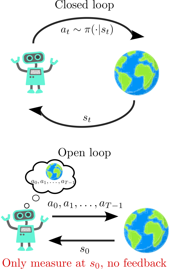
Given a model, solving open-loop OCPs is a well-established field.
But there are also drawbacks in the application to real systems.
- Unforeseen events cannot be accounted for.
- External disturbances/uncertainties are hard/impossible to include.
- Smalles inaccuracies scale exponentially over time.
Question: Can we close the loop around OCPs?

Model predictive control (MPC)

Let us solve the open-loop problem repeatedly on a shorter horizon $p \leq T$.
The “feedback” is setting the initial condition of the OCP.

images/14-optimal-control/open-closed-loop.svg — Inspired by Sergey Levine’s CS285 lecture.

MPC scheme

\[\begin{equation}\text{OCP:}\quad\min_{a_0,\ldots,a_{T-1}} \sum_{t=0}^T \ell(s_t,a_t) = \min_{a_0,\ldots,a_{T-1}} L(a) \quad \text{s.t.}\quad s_{t+1}=f(s_t,a_t),~t=0,1,\ldots,T-1. \tag{\ref{eq:OC_ocp}}\end{equation}\]

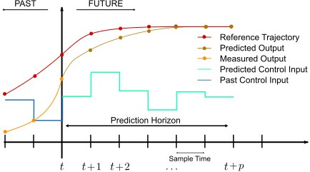
images/14-optimal-control/MPC.svg — Source: Wikipedia.

The MPC loop

Measure system state $s_t$ and use it as the initial state for the OCP $\eqref{eq:OC_ocp}$.
Solve $\eqref{eq:OC_ocp}$ using a model of the real system over a prediction horzion of length $p$.
Apply first entry of $a^*$ (i.e., $a_0^*$) to the real system.
Advance real system by one time step.
Repeat.

Pros and cons

$\textcolor{green}{\mathbf{+}\text{ Very robust.}}$
$\textcolor{green}{\mathbf{+}\text{ No offline learning phase (if model known).}}$
$\textcolor{green}{\mathbf{+}\text{ Easy to include state constraints.}}$
$\textcolor{green}{\mathbf{+}\text{ Lots of theory.}}$ (e.g., (Grüne and Pannek 2017))

$\textcolor{red}{\mathbf{-}\text{ Real-time capability (in particular for nonlinear models).}}$ $\textcolor{red}{\mathbf{-}\text{ Control performance depends on model quality.}}$

Example: Autonomous driving

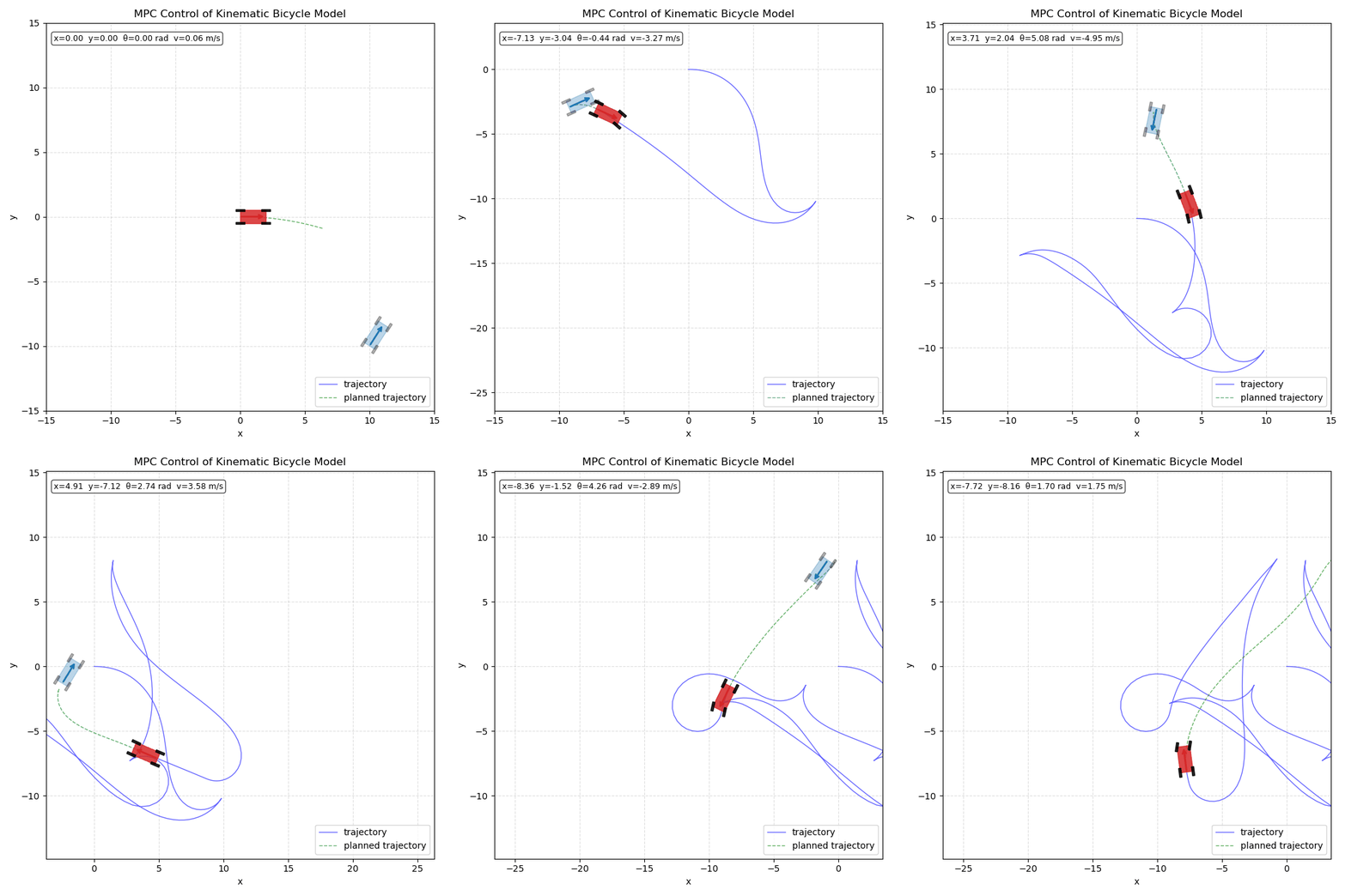
We want to plan the trajectory of an autonomous vehicle from an initial position towards a terminal position.

Dynamics: Simplified kinematic bicycle model (Kong et al. 2015).

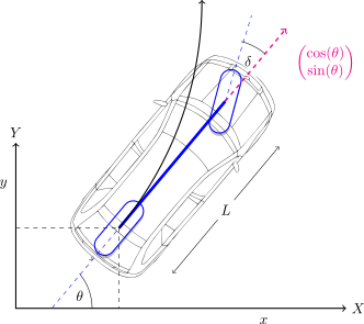
images/14-optimal-control/Bicycle2.svg — Source: Algorithms for Automated Driving.

\[\begin{align*} s&=\begin{bmatrix} x \\ y \\ \theta \\ v \end{bmatrix},~ a=\begin{bmatrix} \mathsf{acc} \\ \delta \end{bmatrix}, \\ \dot{s} &=\begin{bmatrix} s_4 \cos s_3 \\ s_4 \sin s_3 \\ \frac{s_4}{L} \tan a_2 \\ a_1 - \lambda s_4 \end{bmatrix}. \end{align*}\]

Objective: terminal condition to approach target location \[\min_{a_0,\ldots,a_{p-1}} \ell(s_p) = \norm{s_p - s_p^\mathsf{target}}_2^2\quad\text{s.t.}\quad \mathsf{bicycle~model}.\]
Discretization: $\Delta t = 0.2$, $p=25$.

MPC optimization: Adam ($\eta=0.1$); 10 steps.
Results:

Using linearized models in MPC

Approach to avoid the large online cost in many MPC applications: use linearized dynamics instead!
- 💡 This is a very common approach in control theory, in particular linearization around the desired state $s^{\mathsf{target}}$.
Approach via Taylor series expansion around current state $\overline{s}_k, \overline{a}_k$.
Introduce distance to current state: \[\Delta s_t = s_t - \overline{s}_t, \quad \Delta a_t = a_t - \overline{a}_t.\]
First-order (i.e., linear) approximation in $\Delta s_t$ and $\Delta a_t$: \[s_{t+1} \approx \underbrace{f(\overline{s}_t,\overline{a}_t)}_{\fragment{ =\overline{s}_{t+1} }} + \underbrace{\left. \pdiff{f}{s}\right|_{(\overline{s}_t,\overline{a}_t)}}_{\fragment{ =A }} \Delta s_t + \underbrace{\left. \pdiff{f}{a}\right|_{(\overline{s}_t,\overline{a}_t)}}_{\fragment{ =B }} \Delta a_t + \Oc(\Delta s_t^2, \Delta a_t^2)\] \[\begin{equation} s_{t+1} - \overline{s}_{t+1} = \boxed{\Delta s_{t+1} \fragment{ \approx A \Delta s_t + B \Delta a_t. }} \label{eq:OC_MPC_linearized} \end{equation}\]

MPC with linearized dynamics

for $t=0,1,2,\ldots$:
$\quad$ Measure the current state $\overline{s}_t,\overline{a}_t$
$\qquad$ of the real (nonlinear system).
$\quad$ Linearize the system dynamics
$\qquad$ around $\overline{s}_t,\overline{a}_t$ $\Rightarrow$ $\eqref{eq:OC_MPC_linearized}$.
$\quad$ Assemble matrices $\hat{Q}_t$ / $\hat{R}_t$ and $G_t$ / $H_t$.
$\quad$ Solve linear problem $\eqref{eq:OC_ocp_linear2}$.
$\quad$ Apply first entry to real system.

$\qquad\qquad$New bottlenecks:$\qquad$ $\bullet$ The linearization around $\overline{s}_t,\overline{a}_t$ $\qquad$ $\bullet$ Assembly of $\hat{Q}_t$ / $\hat{R}_t$ and $G_t$ / $H_t$.

Relation to reinforcement learning

Trade-offs

Learning a policy offline vs. solving an OCP online.
Expensive training vs. expensive inference.

Approaches in between

Explicit MPC.
Differentiable predictive control (DPC).
Monte-Carlo tree search (MCTS).

Explicit MPC

MPC’s main challenge: large online cost!
Can we avoid this? $\Rightarrow$ Let’s revisit the OCP formulation $\eqref{eq:OC_ocp}$ in the MPC setting: \[\begin{equation} \begin{aligned} &\min_{\tilde{a}} \sum_{\tau=0}^p \ell(\tilde{s}_\tau,\tilde{a}_\tau) \\ \text{s.t.}\quad &\tilde{s}_{\tau+1}=f(\tilde{s}_\tau,\tilde{a}_\tau),~\tilde{s}_0=\textcolor{blue}{s_t}. \end{aligned} \label{eq:OC_mpc} \end{equation}\]
This OCP is parameterized by the initial condition $\textcolor{blue}{s_0}$!
If we solve it for every $s_0\in\Sc$ and explicitly store $a^*(s_0)$ in a library, we can quickly retrieve it in the online phase.
But there are infinitely many $s_0$! 😱
Options:
- Approximate by a finite number of $s_0$.
- Special case: linearity.

The explicit linear-quadratic regulator (Bemporad et al. 2002)

For linear models and quadratic costs, \[\begin{align*} f(s,a)&=As+Ba,\\ \ell(s,a) &= s^\top Q s + a^\top R a, \end{align*}\] the solution space $a^*(s_0)$ for $\eqref{eq:OC_mpc}$ is split into polygons on which the optimal feedback $a^*$ is an affine function of the initial condition $s_0$

Finite number of polygons $\Rightarrow$ finite number of OCPs to solve!
Algorithm for the offline phase:
1. Split the space of initial conditions into polygons $i=1,\ldots,N_p$.
2. Determine coefficients $W^i$ and $b_i$ for the affine feedback law (details in (Bemporad et al. 2002)).
Drawback: Exponential growth of polygons with state dimension $n$.
- Workaround: Replace polygon by deep neural net (Karg and Lucia 2020).

Differentiable predictive control (DPC)

Let’s start with a policy network, just as in policy gradient methods: $a=\mu_\phi(s)$.
Inserting into the right-hand side of our model yields an autonomous system: \[s_{t+1}=f(s_t, \mu_\phi(s_t)).\]
We can now formulate a closed-loop performance criterion: \[L(\phi) = \sum_{t=1}^T \norm{s_t - s_t^\mathsf{target}} + \alpha\norm{\mu_\phi(s_t)}. \]

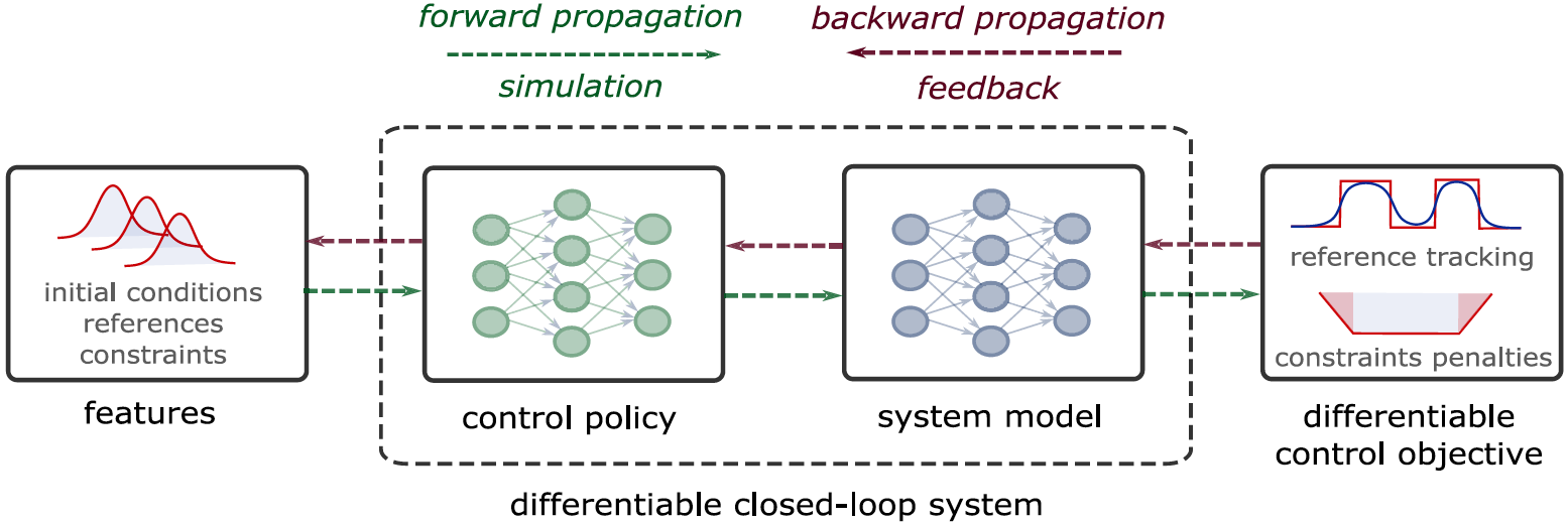
images/14-optimal-control/DPC.png — Differentiable predictive control framework (Drgoňa et al. 2022).

If the dynamics model $f$ (or a learned version $f_\theta$; see next lecture) is differentiable, then we can directly optimize the policy paramter $\phi$ via backpropagation and gradient descent: \[\phi \gets \phi - \eta\diff{L}{\phi}.\]
This is known as differentiable predictive control (DPC).

Summary / what we have learned

Knowing a model of the system dynamics can be very useful, not only for tabular reinforcement learning methods.
Open-loop = Planning: Given an initial condition $s_0$, find the optimal actions for an entire trajectory once.
MPC: Repeated solution of open-loop optimal control problems.
Explicit MPC: Solving the open-loop problem in an offline phase in a parameterized fashion.
Differentiable predictive control (DPC): Policy optimization via direct differentiation through the dynamics model.

References

Bemporad, Alberto, Manfred Morari, Vivek Dua, and Efstratios N. Pistikopoulos. 2002. “The Explicit Linear Quadratic Regulator for Constrained Systems.” Automatica 38 (1): 3–20. doi:https://doi.org/10.1016/S0005-1098(01)00174-1.

Drgoňa, Ján, Karol Kiš, Aaron Tuor, Draguna Vrabie, and Martin Klaučo. 2022. “Differentiable Predictive Control: Deep Learning Alternative to Explicit Model Predictive Control for Unknown Nonlinear Systems.” Journal of Process Control 116: 80–92.

Grüne, L., and J. Pannek. 2017. Nonlinear Model Predictive Control. 2nd ed. Springer International Publishing.

Karg, Benjamin, and Sergio Lucia. 2020. “Efficient Representation and Approximation of Model Predictive Control Laws via Deep Learning.” IEEE Transactions on Cybernetics 50 (9): 3866–78. doi:10.1109/TCYB.2020.2999556.

Kong, Jason, Mark Pfeiffer, Georg Schildbach, and Francesco Borrelli. 2015. “Kinematic and Dynamic Vehicle Models for Autonomous Driving Control Design.” In 2015 IEEE Intelligent Vehicles Symposium (IV), 1094–99. doi:10.1109/IVS.2015.7225830.

Content

Content

Where are we?

Recap: model-based and model-free RL

Algorithm: Value iteration for estimating \(\pi\approx \pi^*\).

Advantages / disadvantages of model-free RL

Today: Can we do better if we know the dynamics?

What is a model?

Types of models

Open-loop optimal control

Planning & optimal control

The deterministic vs. the stochastic case

Stochastic dynamics

Some approaches for stochastic optimal control

Solving the OCP: single shooting

Single shooting

Remaining question:

Gradients in single shooting (1)

Gradients in single shooting (2)

Gradients in single shooting (3)

Gradient calculation in the single shooting method for solving \(\eqref{eq:OC_ocp}\)

Notes

Solving the OCP: full discretization

Comparison: Shooting vs. full discretization

The linear-quadratic case

The linear-quadratic case

Additional conditions

Linear-quadratic optimal control problem

Removing the constraints

Reformulating the cost function

Solving the linear OCP

Some linear algebra

Example: Control of a forklift (1)

Example: Control of a forklift (2)

Closed-loop control

Model predicitve control (MPC)

Model predictive control (MPC)

MPC scheme

The MPC loop

Pros and cons

Example: Autonomous driving

Using linearized models in MPC

MPC with linearized dynamics

Relation to reinforcement learning

Trade-offs

Approaches in between

Explicit MPC

The explicit linear-quadratic regulator (Bemporad et al. 2002)

Differentiable predictive control (DPC)

Summary / what we have learned

References