Deep Reinforcement Learning
Offline Reinforcement Learning
Chair of Safe Autonomous Systems, TU Dortmund
Summer term 2026

Imitation learning
- Two of the biggest challenges in RL:
- Long waiting times until we find a policy that does not fail completely.
- Designing good reward functions that actually make the agent do what we want it to do.
- What can we do to circumvent this?
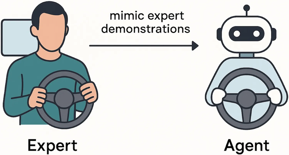
\(\Rightarrow\) “Let’s just show the agent how it’s done?”: learn from an expert! - The concept behind this is imitation learning.
- Given examples from a human expert, try to derive a policy that mimicks this behavior as closely as possible …
- … while generalizing to previously unseen scenarios.
 Source: Medium.com.
 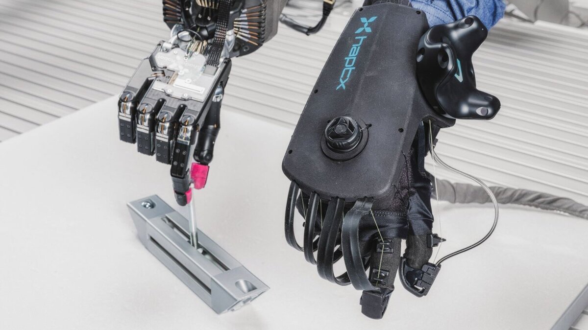 Source: Innovation campus future mobility.
Some developments in imitation learning (2)
Interactive / Human-in-the-Loop IL
- To fix BC’s compounding errors without the cost of IRL, methods like Dataset Aggregation (DAgger, (Ross, Gordon, and Bagnell 2011)) were introduced.
- Runs current policy in the environment.
- When it makes a mistake and goes off-track, an expert intercepts and provides the correct action labels for those erroneous states.
- This data is added back into the training set.
\(\pluspoint\) Directly fixes covariate shift.
\(\pluspoint\) Forces the agent to learn how to recover from its own mistakes.
\(\minuspoint\) Requires an expert to be constantly available and online during training to label data.
\(\minuspoint\) Exhausting for humans and frequently impossible for complex setups.
Generative advarsarial imitation learning (GAIL) (Ho and Ermon 2016)
- Two-player game:
- Generator: the agent trying to mimic the expert policy.
- Discriminator: classifier trying to distinguish between agent and expert trajectories.
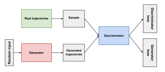
- The discriminator penalizes the agent when it does not create expert-like trajectories.
\(\pluspoint\) Mimicks entire trajectories, not just single transitions as BC.
\(\pluspoint\) No expensive inner loop as in IRL.
\(\pluspoint\) Does not require an interactive expert like DAgger.
\(\minuspoint\) Inherits GAN instabilities (mode collapse, highly sensitive hyperparameters).
\(\minuspoint\) Very data hungry.
Can offline RL work?
- Find the “good stuff” in a dataset full of good and bad behaviors.
Example, consider a dataset of various drivers:
\(\circ\) with imitation learning, we would find the average performance 👎
\(\circ\) with offline RL, we hope to extract a policy mimicking the best driver’s performance in each situation 👍 - Generalization: good behavior in one place may suggest good behavior in another place.
Driving example: we improve upon the best driver by generalizing to unseen situations. - “Stitching”: parts of good behaviors can be recombined.
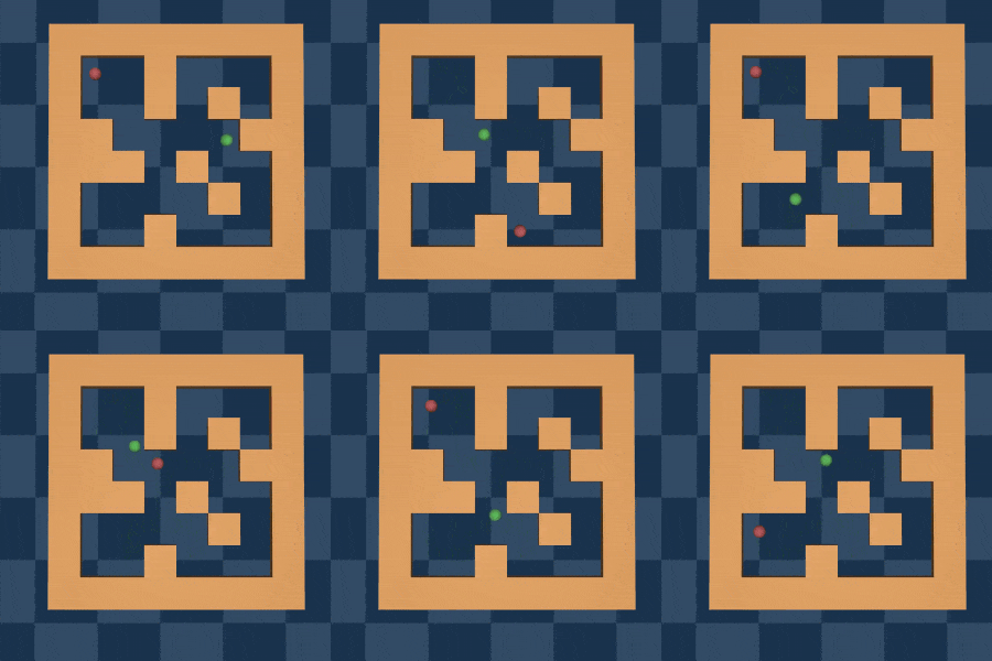
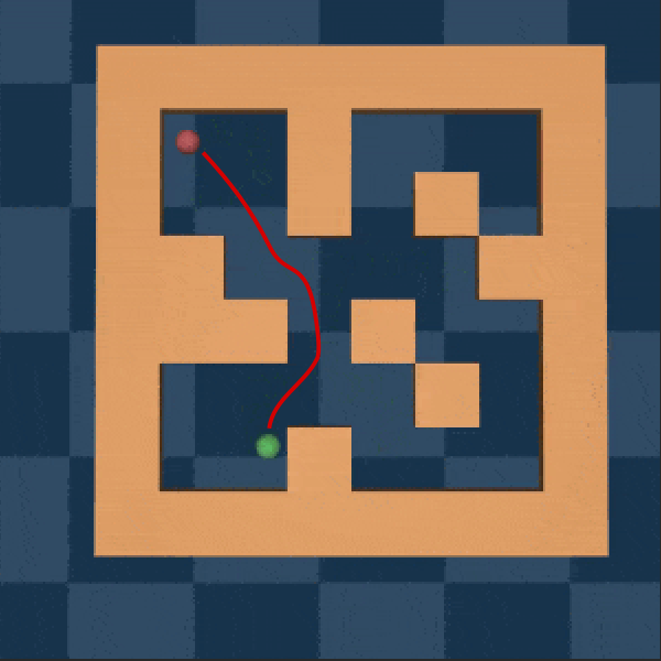
Stitching (Source: Sergey Levine’s CS285 lecture).
Takeaway: It’s not just imitation learning!
Intuition: Get order from chaos.
- On micro scales (e.g., a “straight path” from a bunch of wiggly trajectories).
- On macro scales (e.g., \(A\to B \to C\) \(\Rightarrow\) \(A\to C\)).
Why is offline RL so hard?
Fundamental problem: counterfactual queries
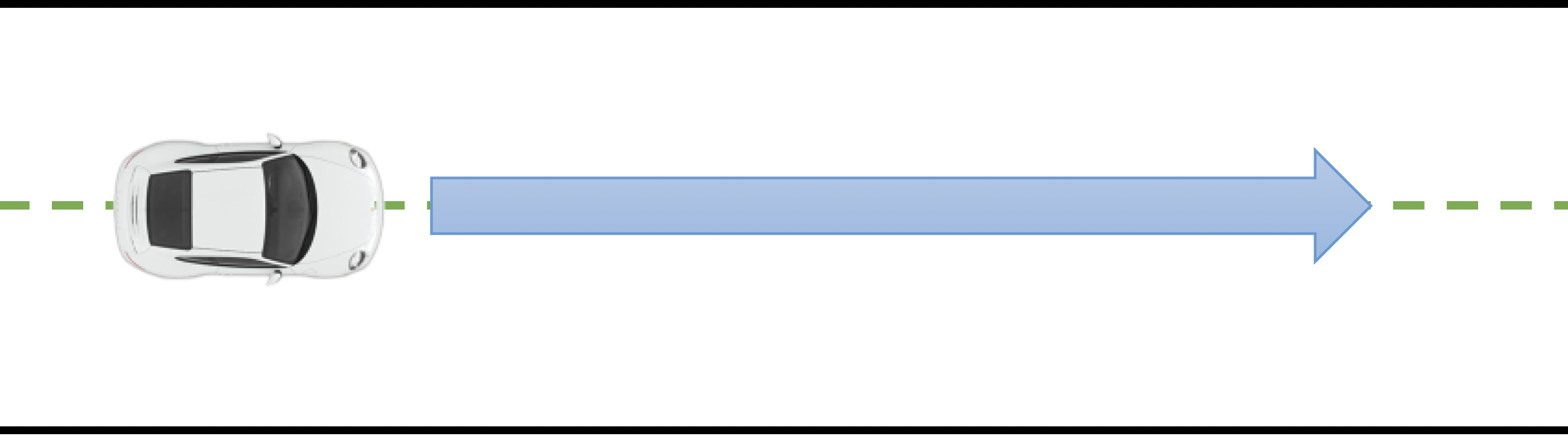
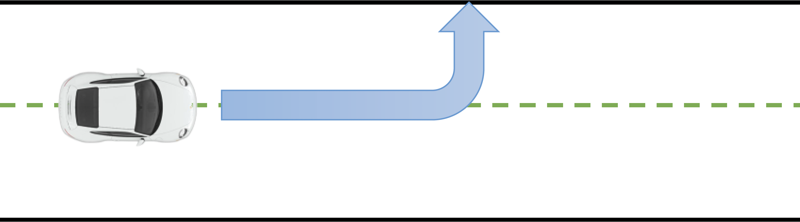
- Is this good or bad?
- How can we know if we have never seen it?
- Online RL algorithms don’t have to handle this.
- They can simply try this action and see what happens.
- Offline RL methods have to account for these unseen (OOD: “out of distribution”) actions,
- ideally in a safe way …
- while still making use of generalization to come up with behaviors that are better than the best thing seen in the data!
Example: Q-learning / Bellman update
\[ Q_\theta \gets r + \gamma \E_{s'\sim \psprimesa}\Big[\underbrace{\max_{a'\in\Ac} Q_{\bar{\theta}}(s',a')}_{\textbf{can go OOD}}\Big] \]
💡 out of distribution vs. out of sample.
- Out of sample \(\Rightarrow\) generalization: Evaluation outside the training dataset, but on data from the same distribution.
- Out of distribution \(\Rightarrow\) Evaluation on unseen data from a different distribution. This is much harder!
Distributional shifts (1)
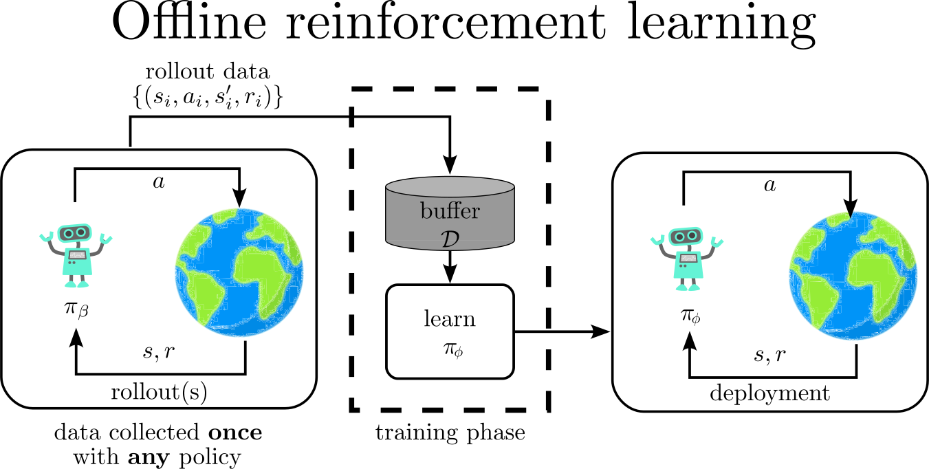
Formally: \[\begin{align*} \Dc &= \set{(s_i,a_i,s'_i,r_i)}_{i=1}^N \\ s &\sim \rho_\beta(s) \\ a &\sim \pi_\beta\agivenb{a}{s} \quad \fragment{ \text{(generally unknown)} } \\ s' &\sim \psprimesa \end{align*}\]
\[\text{RL objective:}\quad \max_\phi \sum_{t=0}^T \Expsub{\gamma^t r_t}{s\sim\rho_\phi, a\sim \piphi\agivenb{\cdot}{s}}\]
- “Model” is valid under \(\pi_\beta\)…
- not under \(\piphi\)!
- “Model” could be the \(Q\)-function \(Q_{\piphi}\),
- or the dynamics \(p_\phi\agivenb{s'}{s,a}\).
Distributional shifts (2)
Example: Empirical risk minimization (maximum likelihood)
\[\theta = \arg\min_{\hat\theta} \Expsub{\cbracket{f_{\hat{\theta}}(x) - y}^2}{x\sim p(x), y\sim p\agivenb{y}{x}}\]
Question: Given some \(x^*\), is \(f(x^*)\) correct?
- \[\Expsub{\cbracket{f_{\hat{\theta}}(x) - y}^2}{x\sim p(x), y\sim p\agivenb{y}{x}} \quad \text{is low}\] \(\Rightarrow\) probably yes.
- \[\Expsub{\cbracket{f_{\hat{\theta}}(x) - y}^2}{x\sim \bar{p}(x), y\sim p\agivenb{y}{x}} \quad \text{is generally not, if} ~ \bar{p}(x) \neq p(x)\] \(\Rightarrow\) probably no.
- What if \(x^* \sim p(x)\)?
- Not necessarily…
- but neural networks tend to generalize well!
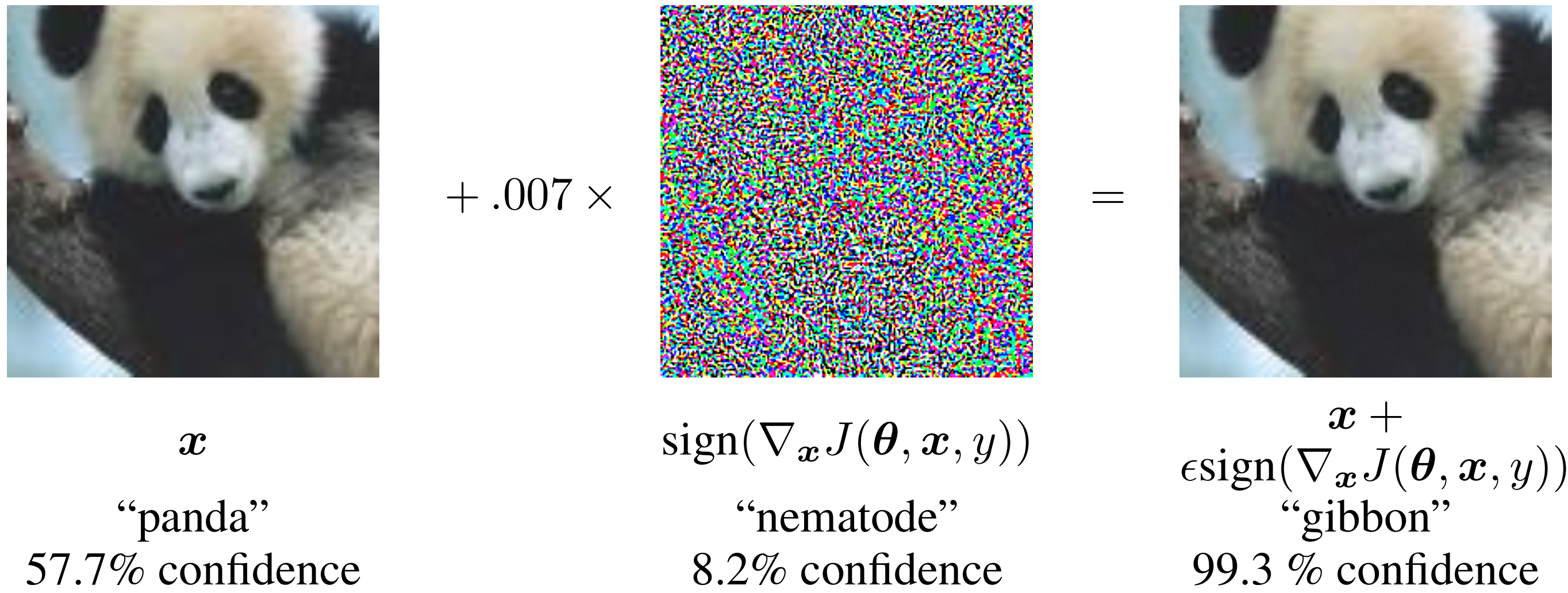
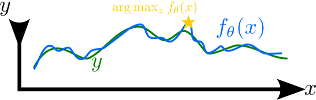
What if we pick the maximizing \(x^*\)?
\[ x^* = \arg\max_x f_\theta(x) \]
💡 This is exactly what we’re exploiting in adversarial learning!
Overestimation bias in offline RL
\(Q\)-learning and \(Q\)-function actor-critic
\[\begin{align*} \phi &= \arg\min_{\hat{\theta}} \Expsub{\norm{Q_\theta(s,a)-y}^2}{s\sim\rho_\beta,a\sim \textcolor{red}{\pi_\beta\agivenb{\cdot}{s}}}, \\ y_i &= r_i + \gamma \Expsub{Q_\theta(s'_i,a')}{s'_i\sim\rho_\beta,a'\sim \textcolor{blue}{\piphi\agivenb{\cdot}{s'_i}}} \end{align*}\]
- Trying to find the best policy: we want \(\textcolor{blue}{\piphi\agivenb{a}{s}} \neq \textcolor{red}{\pi_\beta\agivenb{a}{s}}\)!
- But we only have \(s'_i\) for \(s_i, a_i\) from our offline dataset.
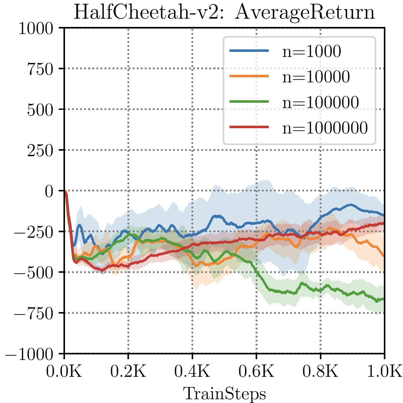
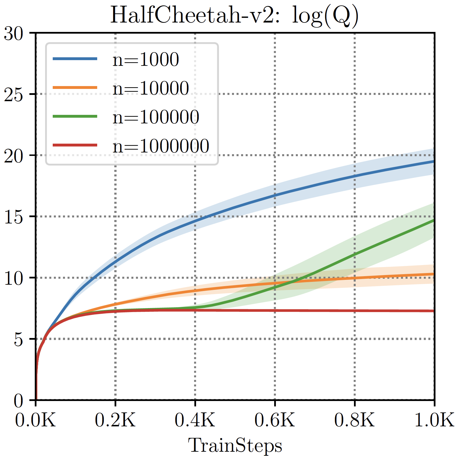
- Even worse: We’re actually picking an adversarial example, \[\phi = \arg\max_{\hat{\phi}} \Expsub{Q_\theta(s,a)}{a\sim \pi_{\hat\phi}\agivenb{\cdot}{s}}.\]
Example: SAC offline RL (Kumar et al. 2019)
Model-based RL
\[f = \arg\min_{\hat f} \Expsub{\norm{f(s,a)-s'}_2^2}{s\sim\rho_\beta,a\sim\textcolor{red}{\pi_\beta\agivenb{\cdot}{s}}, s'\sim \psprimesa} \]
- Probably large: \(\Expsub{\norm{f(s,a)-s'}_2^2}{s\sim\rho_\beta,a\sim\textcolor{blue}{\pi_\phi\agivenb{\cdot}{s}}, s'\sim \psprimesa}.\)
- Even worse: Pick \(\piphi\) to maximize the reward under \(f\)!
Algorithmic evolution of methods
The following strategies (or classes of approaches) are the most common ones today:
- Policy constraint methods: Stay close to the data, e.g., \[ \KLdiv{\piphi\agivenb{\cdot}{s}}{\pi_\beta\agivenb{\cdot}{s}}\leq \epsilon. \]
- Value-regularization & pessimism: Go anywhere, but assume what you haven’t seen is dangerous \(\Rightarrow\) avoid overestimation.
- Implicit \(Q\)-learning: Implicitly define constraints to avoid leaving the support of the behavior policy \(\pi_\beta\).
Common theme: “Maximize return while staying close to the dataset.
How to learn \(\pi_\beta\) if we don’t know it
- Constraining the KL divergence requires knowledge of the behavior policy \(\pi_\beta\).
- What can we do if we don’t know it? \(\Rightarrow\) extract it from the dataset!
Behavior cloning.
- Given a dataset \(\Dc=\set{(s_i,a_i)}_{i=1}^N\), we have a probabilistic supervised learning problem.
- Find the probability distribution \(\pi_\psi\agivenb{a}{s}\) giving rise to \(\Dc\).
- In other words maximize the likelihood of \(a_i\) given \(s_i\) over \(\Dc\).
- Approaches:
\(\circ\) Variational autoencoder (VAE) (Kingma and Welling 2013):
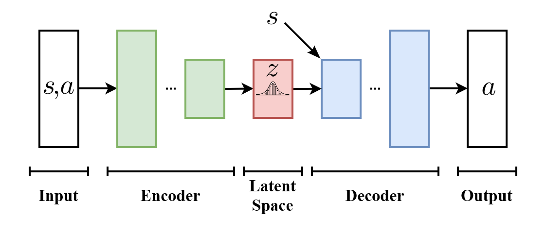 Adapted from Wikipedia.
\(\circ\) Gaussian policy: \(\pi_\psi\agivenb{a}{s} = \Nc(\mu_\psi(s), \sigma^2_\psi(s))\).
\(\circ\) Generative modeling
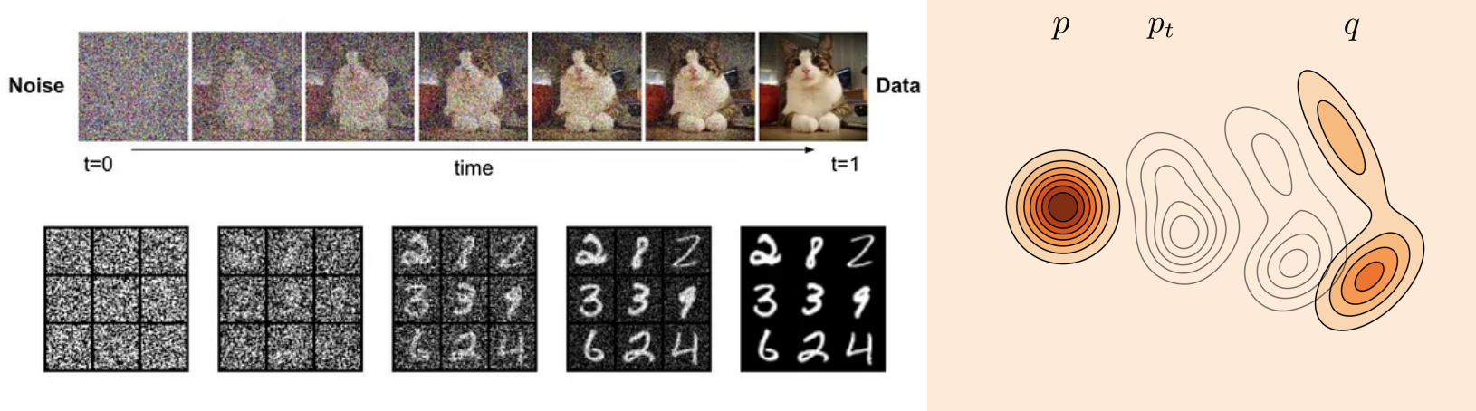 Source: Medium.com.
Conservative \(Q\)-learning
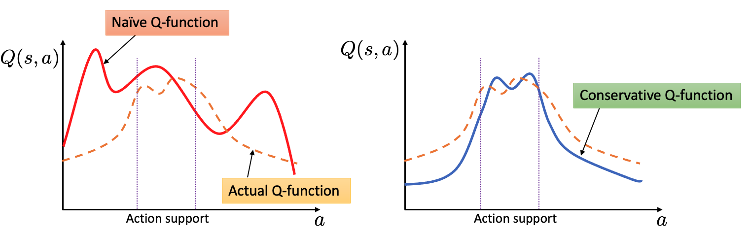
- We have seen that overestimation of \(Q\)-values outside the offline dataset \(\Dc\) is the main source of failure for offline RL.
- Policy constraint methods (previously): Penalize deviations of the policy from the behavior policy \(\pi_\beta\).
- Alternative: Penalize the \(Q\)-function outside \(\Dc\) \(\Rightarrow\) value regularization!
- This is what conservative \(Q\)-learning (CQL, (Kumar et al. 2020)) does:
\(\Rightarrow\) introduce a lower bound (a pessimistic approximation) of the actual \(Q\)-function. - We can then simply use the pessimistic \(Q\)-function in \(Q\)-learning or Actor-Critic methods.
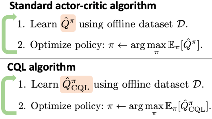
Question: How can we achieve this?
Advantage-weighted regression
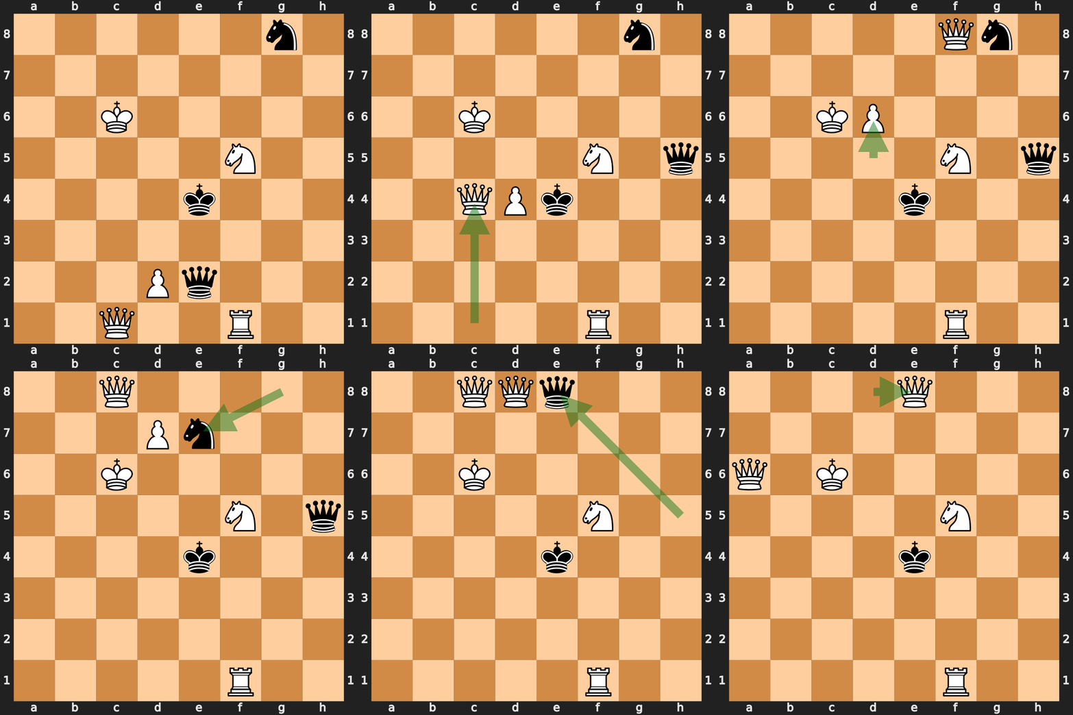
Let’s consider the chess example
- Imagine we are trying to learn how to play chess purely by watching a large database of past games.
- Some games were played by grandmasters, some by mediocre players or even beginners.
- If we copy every move equally (standard Behavior Cloning (BC)), we will become a mediocre player because we are copying the mistakes of the beginners just as much as the great moves of the masters.
- Ideally, we want to copy the actions that led to better-than-expected outcomes and ignore (or suppress) the actions that led to poor outcomes.
Advanted-weighted regression (AWR, (Peng et al. 2019)):
- Imitation learning on the dataset.
- State-action pairs are weighted by an exponential function of the “advantage” (i.e., how much better the action was compared to the average action from that state).
- Can be seen as weighted BC.

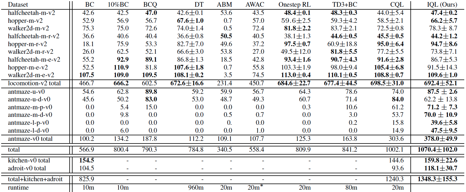
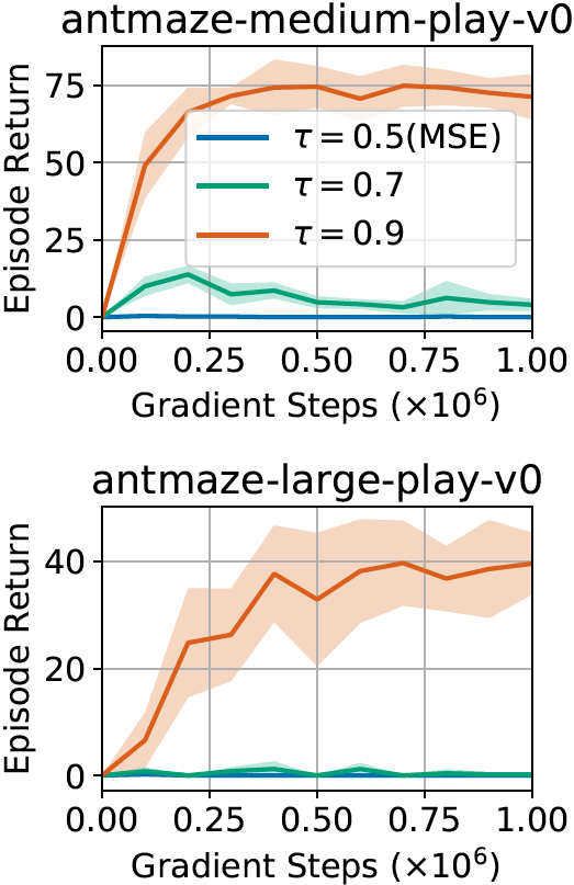
Some results